Chapter 8 Theoretical foundations
8.1 Explaining SLR behavior
This project involves explaining the behavior of an SLR w.r.t. the true LR. Here is a summary of the main results:
- \(|log(LR) - log(SLR)|\) is likely to be unbounded and has to do with the fact that the LR and the SLR typically do not share the same invariances (the contour lines of the LR and SLR differ). The example in the paper shows how this works for univariate Gaussian data and squared Euclidean distance score function.
- Large discrepancies between the LR and the SLR are probably even with univariate data
- The most likely and largest discrepancies between the SLR and LR tend to be when both the LR and SLR are very large or very small.
- Bounds on the tail probabilities of the LR given a score
- Bounded LR implies bounded SLR
- LRs are always larger than the SLR in expectation under the prosecution hypothesis and smaller in expectation under the defense hypothesis (technically the latter statement should be that the inverse of the LR is larger in expectation than the inverse of the SLR)
We submitted this to JRSS Series A, but it was returned to us with the option to resubmit. The biggest issue seemed to be a misunderstanding about whether independence under the prosecution hypothesis is reasonable. Otherwise, the first reviewer seemed to focus heavily on the LR paradigm generally, and they also seemed to misunderstand that our definition of “LR” was of the true distributions from which data are sampled under both hypotheses. To address these misunderstandings, we are completely rewriting the intro to move the focus from LRs to SLRs and correcting some specific lines that may have helped lead to some confusion. We are also taking more time in the paper to discuss that, the specific source problem conditions on the source of the evidence under the prosecution hypothesis, and thus the “dependence” that we think the reviewers are thinking should exist is lost. That is, the fact that the unknown source and known source data should be more similar under \(H_p\) than any random two pieces of evidence is already conditioned upon.
See here for the current draft of the paper from this work.
8.2 Common Source vs Specific Source Comparison via Information Theory
Please note that this project has changed somewhat significantly, but this information might be relevant for others in the future.
See here for the current draft of the paper from this work.
8.2.1 Introduction
Central Goals
- continue work started by Danica and Peter Vergeer on the analysis of likelihood ratios
- study the differences between specific source (SS) and common source (CS) likelihood ratios (LRs) in an information theoretic way
- does the CS or SS LR have more “information”?
- does the data (or the score) have more “information” about the SS or the CS hypothesis?
- can be the CS or SS hypotheses (prosecution or defense) be formally compared in terms of being easier to “prove” or “disprove”?
General Notation Let \(X \in \mathbb{R}^{q_x}\) and \(Y \in \mathbb{R}^{q_y}\) be two random vectors with joint distribution \(P\) and corresponding density \(p\).
- : \(\mathbb{H}(X) = -\int{p(x) \log p(x) dx}\)
- : \(\mathbb{H}(X|Y) = \mathbb{E}_{Y}\left[-\int{p(x|y) \log p(x|y) dx}\right]\)
- : \(\mathbb{H}_{2}(X|Y) = -\int{p(x|y) \log p(x|y) dx}\)
- : \(\mathbb{I}(X;Y) = \mathbb{H}(X) - \mathbb{H}(X|Y)\)
Proof that Mutual Information is always positive:
\[\begin{align*} \mathbb{I}(X;Y) &= \mathbb{H}(X) - \mathbb{H}(X|Y) \\ &= -\int{p(x) \log p(x) dx} + \int{\int{p(x|y)p(y) \log p(x|y) dx} dy} \\ &= -\int{\int{p(x,y) \log p(x) dx}dy} + \int{\int{p(x,y) \log p(x|y) dx} dy} \\ &= -\int{\int{p(x,y) \log p(x) dx}dy} + \int{\int{p(x,y) \log \frac{p(x,y)}{p(y)} dx} dy} \\ &= \int{\int{p(x,y) \log \frac{p(x,y)}{p(x)p(y)} dx}dy} \\ &= KL(P||P_{X} \times P_{Y}) \\ &\geq 0 \end{align*}\]
8.2.2 Common Source vs Specific Source LR
The “common source” problem is to determine whether two pieces of evidence, both with unknown origin, have the same origin. One might be interested in this problem if two crimes were suspected to be linked, but no suspect has yet been identified. Alternatively, the “specific source” problem is to determine whether a fragment of evidence coming from an unknown source, such as evidence at a crime scene, has the same origin as a fragment of evidence of known origin, such as evidence collected directly from a suspect.
Basic Setup
- \(H \in \{ H_p, H_d \}\) as the random variable associated with the CS hypothesis.
- \(A\) and \(B\) are discrete r.v.’s representing two “sources” of evidence
- distributions for \(A\) and \(B\) defined conditionally based on the hypothesis
- SS hypothesis is represented by the conditional random variable \(H|A\)
- \(X\) is data coming from \(A\), \(Y\) is data coming from \(B\)
- compare information contained in \((X,Y)\) about \(H\) and \(H|A\)
- join density can be written as \(p(X,Y,A,B,H) = p(X,Y|A,B)p(B|A,H)p(A|H)p(H)\)
Is there more information in a CS or SS LR?
Let us examine this question in two different ways.
- Is the posterior entropy (given \((X,Y)\)) in the common source hypothesis smaller than that of the specific source hypothesis?
- In other words, would observing the specific value of \(A\) as well as the data make you more certain about \(H\) than just observing the data?
- Is the posterior entropy (given \((X,Y)\)) in the common source hypothesis smaller than the average (over possible values for \((X,Y,A)\)) posterior entropy of the specific source hypothesis?
- In other words, do you expect that, on average, observing the value of \(A\) as well as the data make you more certain about \(H\) than just observing the data?
Answering the first question/interpretation, to me, requires proving that
\[ \mathbb{H}_{2}(H|X,Y) - \mathbb{H}_{2}(H|X,Y, A) \geq 0 \].
Answering the second question requires proving that
\[ \mathbb{H}(H|X,Y) - \mathbb{H}(H|X,Y, A) \geq 0 \].
Luckily, the second question is true due to the fact that
\[\begin{align*} \mathbb{H}(H|X,Y) - \mathbb{H}(H|X,Y,A) &= \mathbb{E}_{(X,Y)} \left[ - \int{p(h,a|x,y) \log p(h|x,y) d(h,a)} + \int{p(h,a|x,y) \log p(h|x,y,a) d(h,a)} \right] \\ &= - \int{p(h,a|x,y)p(x,y) \log \frac{p(h,a|x,y)}{p(a|x,y)p(h|x,y)} d(h,x,y,a)} \\ &= \mathbb{E}_{(X,Y)} \left[ KL(P_{(H,A)|(X,Y)}||P_{H|(X,Y)} \times P_{A|(X,Y)}) \right] \geq 0 \end{align*}\]
Whether or not \(\mathbb{H}_{2}(H|X,Y) - \mathbb{H}_{2}(H|X,Y, A) \geq 0\) is not obvious. We have that
\[\begin{align*} \mathbb{H}_{2}(H|X,Y) - \mathbb{H}_{2}(H|X,Y, A) &= \int{-p(h|x,y)\log p(h|x,y) dh} - \int{-p(h|x,y,a) \log p(h|x,y,a) dh} \\ &= \frac{p(a)}{p(a|x,y)}\int{-p(h|x,y,a)\log p(h|x,y) dh} + \int{p(h|x,y,a) \log p(h|x,y,a) dh}\\ &??? \end{align*}\]
We can try and understand the value of \(\mathbb{H}_{2}(H|X,Y) - \mathbb{H}_{2}(H|X,Y, A)\) in terms of \(\frac{p(a)}{p(a|x,y)}\). For example, if \(\frac{p(a)}{p(a|x,y)} \geq 1\), then \(\mathbb{H}_{2}(H|X,Y) - \mathbb{H}_{2}(H|X,Y, A) \geq 0\). If \(\frac{p(a)}{p(a|x,y)} \leq 1\), then it is hard to say much about the value of \(\mathbb{H}_{2}(H|X,Y) - \mathbb{H}_{2}(H|X,Y, A)\).
Is there more information in the data about the CS or SS hypothesis? Under the second scenario, we can study this question by looking at
8.2.3 Other notions of information
- Information in \(Y\) about \(X\):
- \(\int{p(x|y) \log \frac{p(x|y)}{p(x)} dx}\)
- nonnegative
- Equal to zero when \(X \perp Y\)
- needn’t integrate over \(Y\) (?)
- as opposed to entropy, information in a random variable requires another random variable to be “predicted”… this is fine in our situation as we have a natural candidate: \(H_p\) or \(H_d\)
8.2.4 Information Theoretic Specific Source Score Sufficiency Metric
Consider the specific source problem. The following derivations are very similar to those in the “infinite alternative population” situation considered in the paper that Danica, Alicia, Jarad, and I submitted. Assuming \(X \perp Y|A,B\) and both \(X \perp B|A\) and \(Y \perp A|B\), the LR is
\[\begin{align*} LR &= \frac{p(x,y|A = a,B = a)}{p(x,y|A = a,B \neq a)} \\ &= \frac{p(x|A = a)p(y|A = a, B = a)}{p(x|A = a)p(y|A = a, B \neq a)} \\ &= \frac{p(y|A = a, B = a)}{p(y|A = a, B \neq a)}. \end{align*}\]
Thus, the LR depends only on the evidence from the unknown source, \(Y\). For a given score, \(s\), we can also write the LR in the following way,
\[\begin{align*} LR = \frac{p(y|A = a, B = a)}{p(y|A = a, B \neq a)} &= \frac{p(s|y, A = a)p(y|A = a, B = a)}{p(s|y, A = a)p(y|A = a, B \neq a)} \\ &= \frac{p(s|y, A = a, B = a)p(y|A = a, B = a)}{p(s|y, A = a, B \neq a)p(y|A = a, B \neq a)} \\ &= \frac{p(s,y|A = a, B = a)}{p(s,y|A = a, B \neq a)} \\ &= \frac{p(y|s,A = a, B = a)p(s|A = a, B = a)}{p(y|s,A = a, B \neq a)p(s|A = a, B \neq a)}. \end{align*}\]
Because \(S|Y,A\) is a function only of the known source evidence, \(X\), and because \(X \perp B|A\), we have that \(S \perp B | Y, A\). This means that \(p(s|y, A = a, B = a) = p(s|y, A = a, B \neq a)\).
Using these facts, we can then decompose the KL divergence of the data under the specific source prosecution hypothesis in the following way,
\[\begin{align*} KL(P(X,Y|A &= a, B = a)||P(X,Y|A = a, B \neq a)) = E_{(X,Y)}\left[ \log \frac{p(x,y|A = a,B = a)}{p(x,y|A = a,B \neq a)} | A = a, B = a \right] \\ &= E_{Y}\left[ \log \frac{p(y|A = a,B = a)}{p(y|A = a,B \neq a)} | A = a, B = a \right] \\ &= E_{S}\left[ E_{Y}\left[ \log \frac{p(y|A = a,B = a)}{p(y|A = a,B \neq a)} |s, A = a, B = a \right] \right] \\ &= E_{S}\left[ E_{Y}\left[ \log \frac{p(y|s,A = a,B = a)}{p(y|s,A = a,B \neq a)} + \log \frac{p(s|A = a, B = a)}{p(s|A = a, B \neq a)} |s, A = a, B = a \right] \right] \\ &= E_{S}\left[ E_{Y}\left[ \log \frac{p(y|s,A = a,B = a)}{p(y|s,A = a,B \neq a)}|s, A = a, B = a \right] \right] + E_{S} \left[ \log \frac{p(s|A = a, B = a)}{p(s|A = a, B \neq a)} \right] \\ &= E_{S} \left[ KL(P(Y|S,A = a,B = b) || P(Y|S, A = a, B \neq a)) \right] + KL(P(S|A = a, B = a)||P(S|A = a, B \neq a)). \end{align*}\]
This implies that \(KL(P(X,Y|A = a, B = a)||P(X,Y|A = a, B \neq a)) \geq KL(P(S|A = a, B = a)||P(S|A = a, B \neq a))\).
An additional consequence is that larger values of \(KL(P(S|A = a, B = a)||P(S|A = a, B \neq a))\) imply smaller values of \(E_{S} \left[ KL(P(Y|S,A = a,B = b) || P(Y|S, A = a, B \neq a)) \right]\). Because \(KL(P(Y|S,A = a,B = b) || P(Y|S, A = a, B \neq a))\) is a nonnegative function in terms of \(S\), small values of \(E_{S} \left[ KL(P(Y|S,A = a,B = b) || P(Y|S, A = a, B \neq a)) \right]\) imply small values (in some sense) of \(KL(P(Y|S,A = a,B = b) || P(Y|S, A = a, B \neq a))\). For example, if the expectation is zero, then the (conditional) KL divergence is zero almost everywhere. Zero KL divergence implies that \(P(Y|S,A = a,B = b) = P(Y|S,A = a,B \neq b)\), i.e. \(S\) is sufficient for the specific source hypothesis.
All of this means that \(KL(P(S|A = a, B = a)||P(S|A = a, B \neq a))\) and \(KL(P(S|A = a, B \neq a)||P(S|A = a, B = a))\) are measures of the usefulness of the score which have direct ties to sufficiency. Estimates of these are always computable in practice, and they are intuitive targets to maximize. For example, if the score is a predicted class probability for “match”, the more discriminative the classifier, the more sufficient the score.
8.3 Score-based Likelihood Ratios are not Fundamentally “Incoherent”
Concern has been raised in the literature on LRs about a desirable property supposedly inherently absent from specific-source SLRs. The property, dubbed “coherence”, intuitively says that given two mutually exhaustive hypotheses, \(H_A\) and \(H_B\), the likelihood ratio used to compare hypothesis A to hypothesis B should be the reciprocal of that used to compare hypothesis B to hypothesis A. I will argue that the claims about the inherent incoherency of SLRs is a result of thinking about SLRs too narrowly. Specifically, I will show that the arguments as to why SLRs are incoherent arise through the inappropriate comparison of SLRs based on different score functions. When one appropriately considers a single score function, incoherency is impossible.
8.3.1 Coherence
Denote by \(E \in \mathbb{R}^{n}\) the vector of random variables describing all of the observed evidence or data which will be used to evaluate the relative likelihood of the two hypotheses. Define by \(LR_{i,j} \equiv \frac{p(E|H_i)}{p(E|H_j)}\) the likelihood ratio of hypothesis \(i\) to hypothesis \(j\). The coherency principal is satisfied if
\[ LR_{i,j} = \frac{1}{LR_{j,i}} \].
Likelihood ratios are fundamentally coherent, but what about score-based likelihood ratios? Denote by \(s: \mathbb{R}^n \rightarrow \mathbb{R}^{q}\) a score function mapping the original data to Euclidean space of dimension \(q\) (typically \(q = 1\)). Similar to LRs, denote by \(SLR_{i,j} \equiv \frac{p(s(E)|H_i)}{p(s(E)|H_j)}\) the score-based likelihood ratio comparing hypothesis \(i\) to hypothesis \(j\). Clearly, in this general context SLRs are also coherent.
8.3.2 Problems with arguments showing SLRs are incoherent
Let us examine the arguments presented in [REFS] to the incoherence of SLRs. These arguments stem from an example where there are two known sources of evidence say, source \(A\) and source \(B\), each producing data \(e_A\) and \(e_B\), respectively. Furthermore, assume that we have a third piece of evidence of unknown origin, \(e_u\), which must have come from either \(A\) or \(B\). We then wish to evaluate the support of the data for \(H_A\) or \(H_B\) defined as follows
\[\begin{array}{cc} H_A: & e_u \text{ was generated from source } A \\ H_B: & e_u \text{ was generated from source } B. \end{array}\]
In this case, we have \(LR_{A,B} = \frac{p(e_A, e_B, e_u|H_A)}{p(e_A, e_B, e_u|H_B)}\). We make use of all available data in the formulation of the numerator and denominator densities. Under the assumptions that each fragment of evidence is independent under both hypothesis \(A\) and \(B\) as well as that \(p(e_A,e_B|H_A) = p(e_A,e_B|H_B)\), the LR reduces to \(LR_{A,B} = \frac{p(e_u|H_A)}{p(e_u|H_B)}\). The second assumption is generally acceptable as the source of \(e_u\) ought to have no impact on the distribution of the evidence with known source.
[REFS] then consider possible SLRs for this example. However, they make an assumption that the score is explicitly a function only of two fragments of evidence. That is, assuming the dimension of \(e_i\), \(dim(e_i) = k\), is constant for \(i = A,B,u\), their score maps \(s:\mathbb{R}^k \times \mathbb{R}^k \rightarrow \mathbb{R}\). An common example of such a score is Euclidean distance, i.e. \(s(x,y) = \left[ \sum_{i = 1}^{k}(x_i - y_i)^2 \right]^{1/2}\). Such a score makes perfect sense in a typical specific-source problem context in which only two fragments of evidence are considered: one from the known source and one from the unknown source.
However, when one desires to create an SLR based on this score in this particular example, it is tempting to suggest that the natural SLR is \(SLR_{A,B} = \frac{p(s(e_A,e_u)|H_A)}{p(s(e_A,e_u)|H_B)}\). Yet, the natural SLR if the hypotheses were reversed is \(SLR_{B,A} = \frac{p(s(e_B,e_u)|H_B)}{p(s(e_B,e_u)|H_A)}\). Neither of these SLRs is the reciprocal of the other, and so the specific source SLR appears to be “incoherent”.
This approach, however, should raise a red flag immediately. Why, in the full LR case, do we require that (simplifying model assumptions aside) the numerator and denominator densities be functions of all available data, but the score is not? Furthermore, if we consider these SLRs in the more general context of scores depending on all available data, we see that, in fact, what [REFS] define to be \(SLR_{A,B}\) and \(SLR_{B,A}\) turn out to be two different SLRs depending on two different scores.
For clarity, we will use \(s(\cdot)\) to denote scores which are explicitly functions of all observed data, and we will use \(\delta (\cdot)\) to denote score functions which are only a function of two fragments of evidence/data. Specifically, the score in \(SLR_{A,B}\) is \(s_1(e_u,e_A,e_B) = \delta(e_u,e_A)\) and the score in \(SLR_{B,A}\) is \(s_2(e_u,e_A,e_B) = \delta(e_u,e_B)\). While the functional form of the score in the two SLRs appears to be the same, clearly \(s_1(e_u,e_A,e_B) \neq s_2(e_u,e_A,e_B)\). Thus, the two SLRs are simply two distinct quantities whose relationship needn’t be expected to be related anymore than if one had decided to use two different function forms of \(\delta(\cdot,\cdot)\) in the two separate SLRs.
One might ask how to reasonably construct an SLR which utilizes a (univariate) score other than a similarity metric for two fragments of evidence. One such example in this case would be \(s(e_u, e_A, e_B) = \frac{\delta(e_u,e_A)}{\delta(e_u,e_B)}\). Intuitively, under \(H_A\), the numerator should be larger than the denominator, while under \(H_B\), the opposite should be true.
8.3.3 Example of a coherent SLR in the two source problem
Suppose that our hypotheses are defined such that
\[ \begin{array}{cc} H_A: & e_u \sim N(\mu_A, \sigma^2), e_A \sim N(\mu_A, \sigma^2), e_B \sim N(\mu_B, \sigma^2) \\ H_B: & e_u \sim N(\mu_B, \sigma^2), e_A \sim N(\mu_A, \sigma^2), e_B \sim N(\mu_B, \sigma^2), \end{array} \]
where \(e_u\), \(e_A\), \(e_B\) are mutual independent under both \(H_A\) and \(H_B\). We will examine three different SLRs: \(SLR^{(A)} \equiv \frac{p(s_1(E)|H_A)}{p(s_1(E)|H_B)}\), \(SLR^{(B)} \equiv \frac{p(s_2(E)|H_A)}{p(s_2(E)|H_B)}\), and \(SLR^* \equiv \frac{p(s_3(E)|H_A)}{p(s_3(E)|H_B)}\), where
\[\begin{align*} E &= (e_u, e_A, e_B)^{\top} \\ s_1(E) &= \log \lVert e_u - e_A \rVert^2 \\ s_2(E) &= \log \lVert e_u - e_B \rVert^2 \\ s_3(E) &= \log \frac{\lVert e_u - e_A \rVert^2}{\lVert e_u - e_B \rVert^2} \end{align*}\]
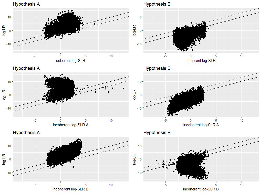
LR versus SLR scatterplots under hypothesis A and B using three types of SLRs: “coherent”, “incoherent” considering hypothesis A first, and “incoherent” considering hypothesis B first.
| RMSE | Exp.Cond.KL | score.KL | true.KL | type | hypothesis |
|---|---|---|---|---|---|
| 3.79 | 2.71 | 1.76 | 4.47 | coherent | A |
| 3.86 | 2.77 | 1.74 | 4.51 | coherent | B |
| 4.64 | 3.37 | 1.10 | 4.47 | incoherent A | A |
| 3.94 | 3.22 | 1.29 | 4.51 | incoherent A | B |
| 3.93 | 3.23 | 1.24 | 4.47 | incoherent B | A |
| 4.73 | 3.44 | 1.07 | 4.51 | incoherent B | B |
8.3.4 Possible Generalizations of Coherent SLRs to the Multisource Case
It might be nice to, in general, be able to construct a reasonable score given a “similarity” score, \(\delta(\cdot, \cdot)\) defined in terms of two pieces of evidence. I’ll propose a couple ways of doing this. First, suppose that instead of two sources, we now have \(K\) sources, one of which is the source of the evidence from an unknown source. The task is to compare the hypothesis that the unknown source evidence was generated by a specific source \(A = a_x \in \mathcal{S} \equiv \{1, 2, ..., K\}\) to the hypothesis that the unknown source evidence was generated by any one of the other sources \(B = b \in \mathcal{S} \setminus a_x\). Mathematically,
\[ \begin{array}{cc} H_A: & e_u \text{ generated by } a_x \\ H_B: & e_u \text{ generated by some } b \in \mathcal{S} \setminus a_x. \end{array} \]
Let’s consider two possible scores, both of which will be based off of an accepted dissimilarity metric, \(\delta(\cdot, \cdot) \geq 0\). The first score that we will consider is
\[ S_1(e_u, e_1, ..., e_K) = \log \frac{\delta(e_u, e_{a_x})}{ \min_{b \in \mathcal{S} \setminus a_x} \delta(e_u, e_b) }. \]
The second score that we will consider is
\[ S_2(e_u, e_1, ..., e_K) = \log \frac{\delta(e_u, e_{a_x})}{ \sum_{b \in \mathcal{S} \setminus a_x} w(b)\delta(e_u, e_b) }, \]
where \(w(b)\) are weights with \(\sum_{b \in \mathcal{S} \setminus a_x} w(b) = 1\). Intuitively, the first score should perform well. The dissimilarity in the numerator should be compared with the smallest dissimilarity in $ a_x$. In the absence of other prior information, only the relative size of the numerator dissimilarity to the smallest dissimilarity of \(b \in \mathcal{S} \setminus a_x\) should matter.
The second score would likely be easier to study in terms of mathematical properties. For example, it might be possible to assume \(E \left[ \delta(e_u, e_i) \right] = \mu_1 < \infty\) if the source of \(e_u\) is that of \(e_i\) but that \(E \left[ \delta(e_u, e_i) \right] = \mu_2 < \infty\) if the sources are different. One might be able to show some type of consistency property if, instead of one copy of \(E = (e_u, e_1, ..., e_K)^{\top}\), we now have \(N\) iid copies \(E_i = (e_u, e_1, ..., e_K)^{\top}_i\). Then, using \(\frac{1}{N} \sum_{i = 1}^{N} \delta(e_{u_i}, e_{j_i})\) in place of \(\delta(e_u, e_j)\) yields the ability to use the law of large numbers. This may be impractical in any real life situation, but I consider the score here nonetheless.
In more generality, there seems to be no reason why a multisource score couldn’t be constructed using an arbitrary summary statistic of the “similarity” scores computed between the unknown source evidence and the alternative population.
8.3.5 Multisource example
For simplicity, we will again assume that all evidence is generated from independent, univariate Gaussian distributions. Specifically,
\[ \begin{array}{ccc} H_p: & e_u \sim N(\mu_K, \sigma^2), & e_i \sim N(\mu_i, \sigma^2), i \in \{ 1,..., K \} \\ H_d: & e_u \sim GMM(\{\mu_k\}_{k = 1}^{K - 1}, \{ \pi_k \}_{k = 1}^{K - 1}, \sigma^2), & e_i \sim N(\mu_i, \sigma^2), i \in \{ 1,...,K \} \end{array}. \]
where all random variables are assumed to be independent conditional on each hypothesis. We will further assume that \(\mu_i \stackrel{iid}{\sim} N(0, \tau^2), i \in \{ 1,..., K-1 \}\).
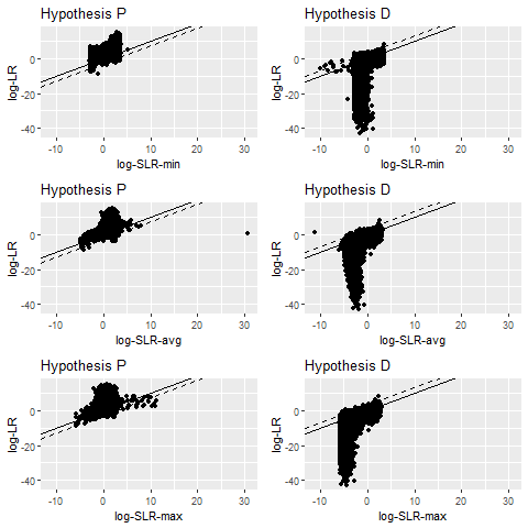
log-LR versus log-SLR scatterplots under hypothesis P and D using three types of SLRs which correspond to using different statistics to aggregate dissimilarity scores in the alternative source population. We try min, average, and max, corresponding to rows 1-3, respectively.Results are based on 10,000 observations for each hypothesis.
| RMSE | Exp.Cond.KL | KL | true.KL | type | hypothesis |
|---|---|---|---|---|---|
| 3.1371 | 2.1718 | 2.2813 | 4.4527 | min | P |
| 8.4669 | 5.1396 | 1.8487 | 6.9865 | min | D |
| 3.4835 | 2.3965 | 2.0568 | 4.4527 | avg | P |
| 7.6549 | 4.2336 | 2.7529 | 6.9865 | avg | D |
| 3.8587 | 2.7198 | 1.7333 | 4.4527 | max | P |
| 7.0711 | 4.1623 | 2.8250 | 6.9865 | max | D |

log-LR versus log-SLR scatterplots under hypothesis P and D using four types of SLRs. The first three scores correspond to using different statistics to aggregate dissimilarity scores in the alternative source population. The fourth score is essentially the predicted probability of Hypothesis P being true given the first three scores based on a sparse Gaussian process model. We try min, average, and max, corresponding to rows 1-3, respectively. Results are based on 1,000 observations for each hypothesis due to training time for the sparse Gaussian process.
| RMSE | Exp.Cond.KL | KL | true.KL | type | hypothesis | |
|---|---|---|---|---|---|---|
| 1 | 3.0605 | 2.0616 | 2.3206 | 4.3809 | min | P |
| 3 | 3.2725 | 2.0710 | 2.3111 | 4.3809 | avg | P |
| 5 | 3.7826 | 2.5398 | 1.8424 | 4.3809 | max | P |
| 7 | 2.6095 | 1.5380 | 2.8442 | 4.3809 | gp | P |
| RMSE | Exp.Cond.KL | KL | true.KL | type | hypothesis | |
|---|---|---|---|---|---|---|
| 2 | 7.9189 | 4.7271 | 2.1101 | 6.8364 | min | D |
| 4 | 7.1000 | 3.8640 | 2.9724 | 6.8364 | avg | D |
| 6 | 6.6734 | 4.0090 | 2.8274 | 6.8364 | max | D |
| 8 | 6.9872 | 3.3887 | 3.4414 | 6.8364 | gp | D |
Aggregating scores via the sparse GP results in a final score that uniformly beats each of the other scores under both the prosecution and defense hypotheses in terms of the score KL divergence.
8.3.6 Other Possible Viewpoints?
I have assumed in the previous section that the order of consideration of hypotheses should not affect the ordering of the data vector \(E = (e_u,e_A,e_B)\) or of the ordering of these arguments to the score function. This seems reasonable, but perhaps [REFS] would argue that considering \(H_A\) first, \(E = (e_u, e_A, e_B)\) and \(s(E) = s(e_u, e_A, e_B)\), but considering \(H_B\) first, \(E = (e_u, e_B, e_A)\) and \(s(E) = s(e_u, e_B, e_A)\). In this case, \(SLR_{A,B} \neq \frac{1}{SLR_{B,A}}\) because we switch the order of arguments to the score from one SLR to the other. Note that, however, if we relax the independence assumptions of independence under either \(H_A\) or \(H_B\), then even the LR becomes “incoherent” because \(\frac{p(e_u, e_A, e_B|H_A)}{p(e_u, e_A, e_B|H_B)} \neq \frac{p(e_u, e_B, e_A|H_A)}{p(e_u, e_B, e_A|H_B)}\) in general.
It is true that the LR depends only on the evidence of the unknown source in this specific scenario, but that is a consequence of modeling assumptions and not of LR paradigmatic principals.
8.4 Copper Wire Synthetic Data
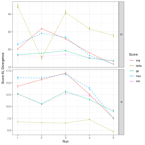
Score KL divergences and Monte Carlo standard errors for five randomly generated synthetic copper wire data sets under \(H_p\) and \(H_d\).
8.5 Optimal matching problem
8.5.1 Two groups case.
Suppose there are two groups \(\pi_{1}\) and \(\pi_{2}\) with densities \(f_{1}(x)\) and \(f_{2}(x)\) on the support \(x \in T\). Let \(p_{1}\) and \(p_{2}\) be the prior probabilities of groups \(\pi_{1}\) and \(\pi_{2}\), respectively. There are new observations \(\mbox{obs}_{1}\) and \(\mbox{obs}_{2}\) with measurements \(x_{1}\) and \(x_{2}\), respectively. The goal is to distinguish there the new observations are from the same group or not. That is to partition the space \(T \times T\) in to \(T_{m} \cup T_{nm}\), where we conclude \(\mbox{obs}_{1}\) and \(\mbox{obs}_{2}\) are from the same group if \((x_{1}, x_{2})\) falls into \(T_{m}\); and otherwise if \((x_{1}, x_{2}) \in T_{nm}\). The two type errors:
- Matching error: \((x_{1}, x_{2}) \in T_{m}\) if \(\mbox{obs}_{1} \in \pi_{1}, \mbox{obs}_{2} \in \pi_{2}\) or \(\mbox{obs}_{1} \in \pi_{2}, \mbox{obs}_{2} \in \pi_{1}\);
- Unmatching error: \((x_{1}, x_{2}) \in T_{um}\) if \(\mbox{obs}_{1}, \mbox{obs}_{2} \in \pi_{1}\) or \(\mbox{obs}_{1}, \mbox{obs}_{2} \in \pi_{2}\).
The probability of errors are: \[P(\mbox{Matching error}) = \int_{T_{m}} \{f_{1}(x_{1})f_{2}(x_{2}) + f_{2}(x_{1})f_{1}(x_{2})\}p_{1}p_{2}dx_{1}dx_{2},\] \[P(\mbox{Unmatching error}) = \int_{T_{um}} \{f_{1}(x_{1})f_{1}(x_{2})p_{1}^{2} + f_{2}(x_{1})f_{2}(x_{2})p_{2}^{2}\}dx_{1}dx_{2}.\] Consider the unweighted sum of those two error probabilities \(P(\mbox{error}) = P(\mbox{Matching error}) + P(\mbox{Unmatching error})\). We have \[P(\mbox{error}) = \int_{T_{m}} \big[\{f_{1}(x_{1})f_{2}(x_{2}) + f_{2}(x_{1})f_{1}(x_{2})\}p_{1}p_{2} - \{f_{1}(x_{1})f_{1}(x_{2})p_{1}^{2} + f_{2}(x_{1})f_{2}(x_{2})p_{2}^{2}\}\big]dx_{1}dx_{2} + C,\] where \(C\) is a constant.
The minimum of this error probability with respect to \(T_{m}\) occurs when \[\begin{equation} T_{m} = \bigg\{(x_{1}, x_{2}): \frac{[f_{1}(x_{1})f_{2}(x_{2}) + f_{2}(x_{1})f_{1}(x_{2})]p_{1}p_{2}}{f_{1}(x_{1})f_{1}(x_{2})p_{1}^{2} + f_{2}(x_{1})f_{2}(x_{2})p_{2}^{2}} < 1 \bigg\}. \label{eq:Optimalrule1} \end{equation}\] This decision region is the optimal matching rule to minimize the probability of the matching errors. Note that \[f_{1}(x_{1})f_{1}(x_{2})p_{1}^{2} + f_{2}(x_{1})f_{2}(x_{2})p_{2}^{2} - [f_{1}(x_{1})f_{2}(x_{2}) + f_{2}(x_{1})f_{1}(x_{2})]p_{1}p_{2} = \{f_{1}(x_{1})p_{1} - f_{2}(x_{1})p_{2}\}\{f_{1}(x_{2})p_{1} - f_{2}(x_{2})p_{2}\}.\] The optimal region \(T_{m}\) in (\(\ref{eq:Optimalrule1}\)) is equivalent to \[\begin{eqnarray} \frac{f_{1}(x_{1})}{f_{2}(x_{1})} < \frac{p_{2}}{p_{1}} &\mbox{and}& \frac{f_{1}(x_{2})}{f_{2}(x_{2})} < \frac{p_{2}}{p_{1}} \ \mbox{ or } \nonumber \\ \frac{f_{1}(x_{1})}{f_{2}(x_{1})} > \frac{p_{2}}{p_{1}} &\mbox{and}& \frac{f_{1}(x_{2})}{f_{2}(x_{2})} > \frac{p_{2}}{p_{1}}, \label{eq:Optimalrule2} \end{eqnarray}\] which corresponds to the optimal classification rule. From (\(\ref{eq:Optimalrule2}\)), the optimal matching rule is equivalent to the optimal classification rule as long as we conclude the observations matched from one group if they are classified to the same group.
Normal distribution. As an example, assume \(\pi_{1}\) and \(\pi_{2}\) are from normal distributions with mean \(\mu_{1}\) and \(\mu_{2}\), and covariance \(\Sigma\). Further assume the prioir probabilities are the same \(p_{1} = p_{2} = 1 / 2\). The optimal decision is to classify \(x_{1}\) and \(x_{2}\) into the same group if \[\begin{equation} \frac{\exp\big[ \{x_{2} - (\mu_{1} + \mu_{2}) / 2\} \Sigma^{-1} (\mu_{2} - \mu_{1}) \big] + \exp\big[ \{x_{1} - (\mu_{1} + \mu_{2}) / 2\} \Sigma^{-1} (\mu_{2} - \mu_{1}) \big]} {1 + \exp\big[ \{x_{1} + x_{2} - (\mu_{1} + \mu_{2})\}' \Sigma^{-1} (\mu_{2} - \mu_{1}) \big]} < 1. \label{eq:OptimalruleNormal1} \end{equation}\] It can be shown that the above inequality is equivalent to \[\begin{eqnarray} \exp\big[ \{x_{2} - (\mu_{1} + \mu_{2}) / 2\} \Sigma^{-1} (\mu_{2} - \mu_{1}) \big] < 1 &\mbox{and}& \exp\big[ \{x_{1} - (\mu_{1} + \mu_{2}) / 2\} \Sigma^{-1} (\mu_{2} - \mu_{1}) \big] < 1 \ \mbox{ or } \nonumber \\ \exp\big[ \{x_{2} - (\mu_{1} + \mu_{2}) / 2\} \Sigma^{-1} (\mu_{2} - \mu_{1}) \big] > 1 &\mbox{and}& \exp\big[ \{x_{1} - (\mu_{1} + \mu_{2}) / 2\} \Sigma^{-1} (\mu_{2} - \mu_{1}) \big] > 1 \label{eq:OptimalruleNormal2} \end{eqnarray}\] For discriminat analysis, it is well known that the optimal classification rule under normal distribution is to classify \(x_{1}\) and \(x_{2}\) to \(\pi_{1}\) if \(\{x_{1} - (\mu_{1} + \mu_{2}) / 2\} \Sigma^{-1} (\mu_{2} - \mu_{1}) \leq 0\) and \(\{x_{2} - (\mu_{1} + \mu_{2}) / 2\} \Sigma^{-1} (\mu_{2} - \mu_{1}) \leq 0\) respectively, and classify them to \(\pi_{2}\) if otherwise.
Feature difference is a method to solve the matching problem via classification. Take \(d = x_{1} - x_{2}\) as the pairwise difference between two observations. It is clear that \(d \sim N(0, 2 \Sigma)\) if \(x_{1}\) and \(x_{2}\) are both from either \(\pi_{1}\) or \(\pi_{2}\), and \(d \sim N(\mu_{1} - \mu_{2}, 2 \Sigma)\) or \(d \sim N(\mu_{2} - \mu_{1}, 2 \Sigma)\) if \(x_{1}\) and \(x_{2}\) are from different groups. Let \(f_{m}(d)\) and \(f_{um}(d)\) be the density of \(d\) if two observations are from the same group and different groups, respectively. Then, \(f_{m}(d)\) is the normal density with mean \(0\) and covariance \(2 \Sigma\), and \(f_{um}(d)\) is the mixture normal \(0.5 N(\mu_{1} - \mu_{2}, 2 \Sigma) + 0.5 N(\mu_{2} - \mu_{1}, 2 \Sigma)\). The optimal discriminant rule is to classify \(d\) into the unmatching case if \[\frac{f_{um}(d)}{f_{m}(d)} = \frac{\exp\{-(d - \mu_{1} + \mu_{2})' \Sigma^{-1} (d - \mu_{1} + \mu_{2}) / 4\} + \exp\{-(d + \mu_{1} - \mu_{2})' \Sigma^{-1} (d + \mu_{1} - \mu_{2}) / 4\}}{2 \exp(-d' \Sigma^{-1} d / 4)} > \frac{p_{1}^{2} + p_{2}^{2}}{2 p_{1} p_{2}}.\] Let \(\mu_{d} = \mu_{1} - \mu_{2}\). The above inequality is equivalent to \[\exp(d' \Sigma^{-1} \mu_{d} / 2) + \exp( - d' \Sigma^{-1} \mu_{d} / 2) > \exp(\mu_{d}' \Sigma^{-1} \mu_{d} / 4) \frac{p_{1}^{2} + p_{2}^{2}}{p_{1}p_{2}},\] which is approximately equivalent to \[|d' \Sigma^{-1} \mu_{d}| / 2 > \mu_{d}' \Sigma^{-1} \mu_{d} / 4 + \log (p_{1}^{2} + p_{2}^{2}) - \log(p_{1}p_{2}).\]
As an illustration, consider one dimensional feature space. Take \(\mu_{1} = 1, \mu_{2} = -1, \Sigma = 1\), and \(p_{1} = p_{2} = 0.5\). Figure 1 shows the optimal matching rule and the optimal rule based on feature difference. We see that in this example the matching region from the feature difference method only overlaps a small fraction of that from the optimal matching rule, and there is a missing alignment for the feature difference method in the two small triangles at the origin. We also note that even though most of the pink area and the blue area in Figure 1 don’t overlap, the probabilities that the pair of data \((x_{1}, x_{2})\) falling into those non-overlapping regions could be small, especially if the absolute value of either coordinate is large. See the contours of multivariate normal distribution in Figure 1.
## Error in library(tidyverse): there is no package called 'tidyverse'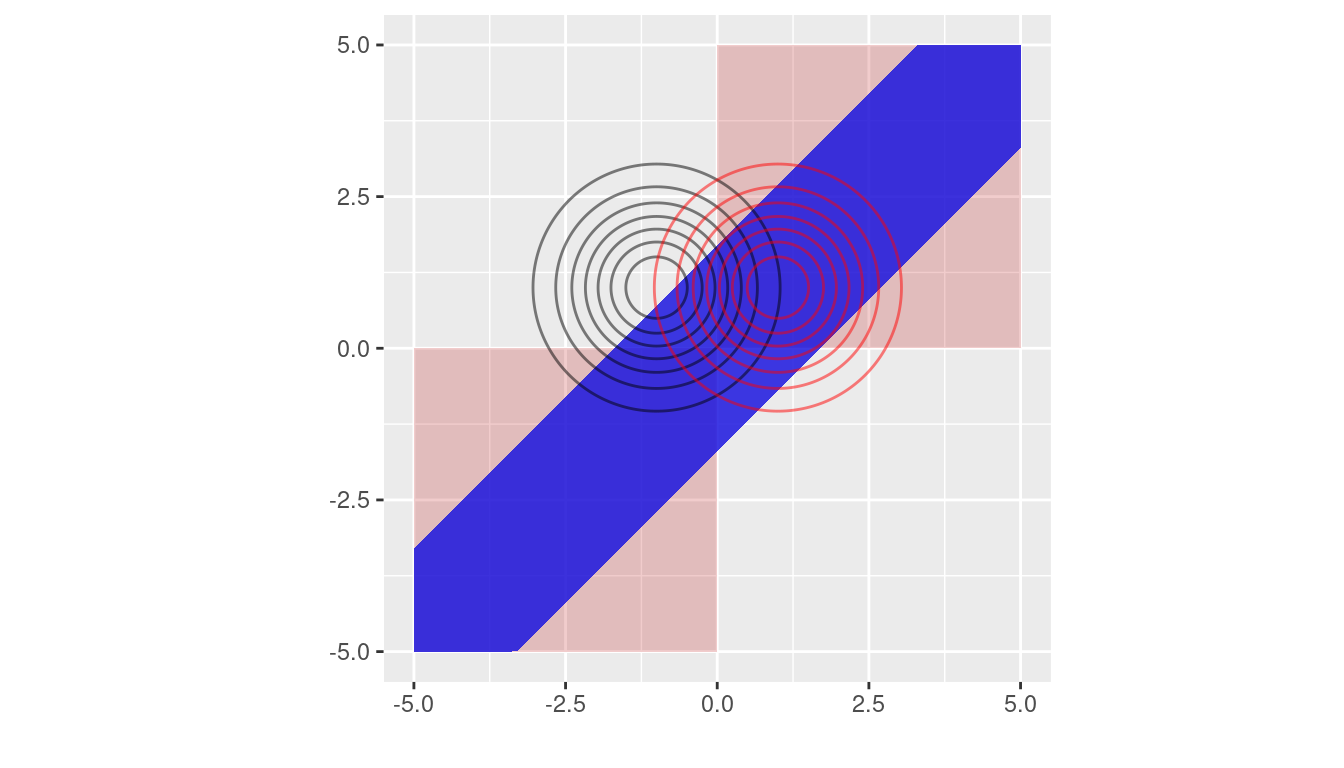
Figure 8.1: Matching regions from the optimal rule (in pink) and the method based on feature difference (in blue). The contours of multivariate normal distribution with means \((1, -1)\) (unmatching case) and \((1, 1)\) (matching case) are marked in black and red, respectively, where the covariance is identity.
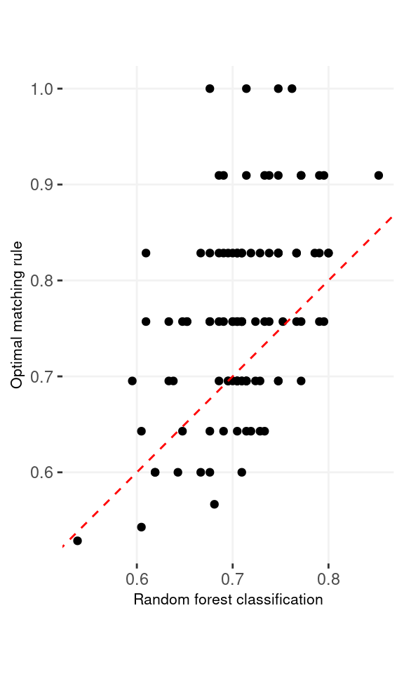
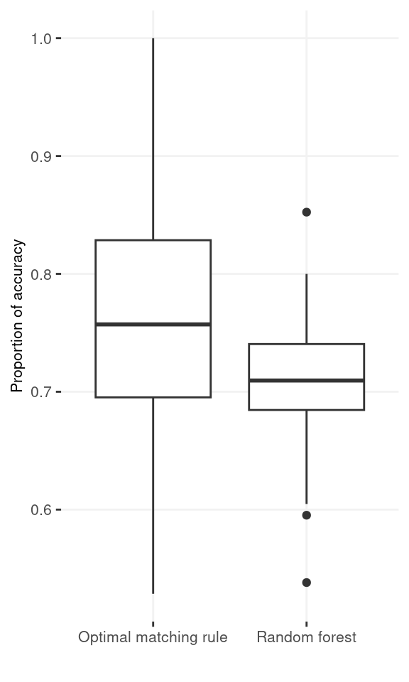
Comparison with random forest. We also conducted a small scale simulation to compare the optimal matching rule with the random forest method applied on the feature difference. The traning data include 50 observations from \(N(1, 1)\) and \(N(-1, 1)\). There are additional 10 observations from each of the group serving as the testing data. We evaluate the percentage of the matching errors on the pairs of the testing data. We repeated the whole simulation 100 times. The accuracy rates are 0.762 and 0.708 for the optimal matching rule and the random forest applied on the differences of the measurements, respectively. 65% out of the 100 repetitions, the former method has higher accuracy than the latter method.
8.5.2 Topics needs exploration
- How to quantify the matching error rates when the training data only inlcude a small part of many potential groups?
- How training errors change as more and more features are collected (dimension \(p\) increases), where only a small fraction of those features carry useful signals (feature selection).
8.5.3 Brief introduction to optimal rule
Suppose that there are multiple sources denoted by \(\pi_g\) for \(g = 1,\ \cdots,\ G\), and observations from each \(\pi_g\) follow a distribution denoted by \(f(\cdot|\pi_g)\). As an example, the figure below shows three different normal distributions by source. Let’s say we have \(n\) observations from those souces but do not know which sources they actually belong to. Our goal is to identify if two observations represented by \(x\) and \(y\) would have come from the same sources or not.
For \(n\) independent observations, \({n \choose 2}\) pairwise comparisons occur. When we sampled 300 observations from each density in the plot above, the following plot illustrates whether each pair actually come from the same sources or not. Blue dots represent the pairs from the same sources, and red ones indicates the pairs from the different sources. If we can predict the blue area accurately as much as possible, our goal to predict the membership of pairwise observations will be attained.
Figure 8.2: True membership of pairs
The following figure displays the optimal rule’s matching results using the data from the previous plot. Likewise, the blue dots represent the matched zone by optimal rule where the pairs are predicted to be from the same sources, and the red ones represent the unmatched zone by optimal rule where the pairs are predicted to be from different sources.
Figure 8.3: Membership of pairs predicted by optimal rule
Now, let \(T_{SS}\) and \(T_{DS}\) denote the same source zone, and a different source zone, respectively where \(T_{SS} \cup T_{DS} = T \times T\), \(T\) is the support of observations, and \(T_{SS} \cap T_{DS} = \emptyset\). With the notation, if a pair, \((x,y) \in T_{SS}\), then they are said to be matched. Otherewise, \((x,y) \in T_{DS}\), which means that the pair is not matching, unmatched. In addition, let \(\pi_X\) and \(\pi_Y\) denote the sources for \(x\), and \(y\), two observations in a pair. Our prior belief for sources is denoted by \(p_g\) for a source, \(\pi_g\), such that the probability of an observation belonging to \(\pi_g\) is equal to \(p_g\), and \(\sum_{g=1}^G p_g = 1\) where \(G\) is the total number of sources considered.
Optimal rule is constructed to minimize the total error occuring when matching the memberships of two observations. The total error probability can be written as the following:
\(\begin{aligned} &P(\mbox{total error}) \\ &=P(\mbox{Incorrectly matching pairs})\\ &=P(\mbox{A pair of observations matched when they are from different sources}) \ +\\ &\ \ \ \ \ \ \ \ P(\mbox{A pair of observations unmatched when they are from the same sources})\\ &= P\left((X,Y) \in T_{SS}|\pi_X \ne \pi_Y\right)P\left(\pi_X \ne \pi_Y \right) + P\left((X,Y) \in T_{DS}|\pi_X = \pi_Y\right)P\left(\pi_X = \pi_Y \right) \\ &=\int_{T_{SS}} \sum_{g_1 \ne g_2}^G f_X(x|\pi_{g_1}) f_Y(y|\pi_{g_2}) p_{g_1}p_{g_2} dx dy + \sum_{g=1}^G p_g^2 - \int_{T_{SS}}\sum_{g=1}^G f_X(x|\pi_{g_1}) f_Y(y|\pi_{g_2}) p_g^2 dxdy \\ &= \int_{T_{SS}} \left[\sum_{g_1 \ne g_2}^G f_X(x|\pi_{g_1}) f_Y(y|\pi_{g_2}) p_{g_1}p_{g_2}\right] - \left[\sum_{g=1}^G f_X(x| \pi_{g}) f_Y(y| \pi_{g}) p_g^2\right] dx dy + C \\ &\mbox{where } C = \sum_{g=1}^G p_g^2 = P(\pi_X = \pi_Y) \mbox{ is a constant over } T_{SS}. \end{aligned}\)
If we could collect every \((x,y) \in T \times T\) such that \[\left[\sum_{g_1 \ne g_2}^G f_X(x|\pi_{g_1}) f_Y(y|\pi_{g_2}) p_{g_1}p_{g_2}\right] - \left[\sum_{g=1}^G f_X(x| \pi_{g}) f_Y(y| \pi_{g}) p_g^2\right] < 0,\] then over the set denoted by \(T_{SS}^{Opt}\), the intergral will attain its minimum, so does \(P(\mbox{total error})\). That is, \[T_{SS}^{Opt} = \underset{T_{SS}}{\mathrm{argmin}} \ P(\mbox{total error}).\]
Note above that the parameters for true densities are unknown in practice, so parameters will be replaced with sample estimates. (e.g., sample mean, and sample variance)
8.5.4 Optimal rule for matching problems
We would like to statistically tell if two observations would have com from the same source or not, which is said to be matching problems. The optimal rule is designed to deal with matching problems, and to minimize the matching error rate defined as the unweighted or weighted sum of the probabilities related to mismatching the memberships of two observations.
Let \(X\) and \(Y\) be two independent random variables associated with the observations \(x\) and \(y\), respectively, and \(T\) be the support of them. i.e., \(x \in T\), \(y \in T\), and \((x,y)\in T \times T\). Suppose that there are \(G\) known sources denoted by \(\pi_1,\ \pi_2,\ \cdots ,\ \pi_G\) with corresponding prior probabilities denoted by \(p_g \in (0,1)\) for \(g = 1,\ \cdots,\ G\) where \(\sum_{g=1}^G p_g = 1\). Next, let \(\pi_X\) and \(\pi_Y\) denote the source of \(X\) and \(Y\). Then, the conditional pdf of \(X\) if it is from a source \(\pi_g\) can be defined as \(f_X(x|\pi_g)\) with the prior probability, \(p_g = P(\pi_X = \pi_g)\). Likewise, the conditional pdf of \(Y\) if it is from a source \(\pi_{g'}\) is written as \(f_Y(y|\pi_{g'})\) with the prior probability, \(p_{g'} = P(\pi_Y = \pi_{g'})\). Lastly, let \(T_{SS}\) and \(T_{DS}\) be the zone for the same sources and zone for the different sources such that \(T_{SS} \cup T_{DS} = T \times T\), and \(T_{SS} \cap T_{DS} = \emptyset\).
Now, we can define two errors occurring in matching problems using the notation above:
- The same source error: \(\pi_X = \pi_g\) and \(\pi_Y = \pi_{g'}\) for \(g \ne g'\), but \((x,y) \in T_{SS}\);
- Different source error: \(\pi_X = \pi_Y = \pi_g\) for some \(g\), but \((x,y) \in T_{DS}\).
It follows that the probabilities of those errors above are given as the following:
\(\pi_X = \pi_g\) and \(\pi_Y = \pi_{g'}\) for \(g \ne g'\), but \((x,y) \in T_{SS}\):
\(\begin{aligned} P(\mbox{The same source error}) &= P\left((X,Y) \in T_{SS}|\pi_X \ne \pi_Y\right)P\left(\pi_X \ne \pi_Y \right)\\ &= \sum_{g_1 \ne g_2}^G \int_{T_{SS}} f_X(x|\pi_{g_1}) f_Y(y|\pi_{g_2}) p_{g_1}p_{g_2} dx dy \\ &= \int_{T_{SS}} \sum_{g_1 \ne g_2}^G f_X(x|\pi_{g_1}) f_Y(y| \pi_{g_2}) p_{g_1}p_{g_2} dx dy, \end{aligned}\)
\(\pi_X = \pi_Y = \pi_g\) for some \(g\), but \((x,y) \in T_{DS}\):
\(\begin{aligned} P(\mbox{different source error}) &= P\left((X,Y) \in T_{DS}|\pi_X = \pi_Y\right)P\left(\pi_X = \pi_Y \right)\\ &= \sum_{g=1}^G \int_{T_{DS}} f_X(x| \pi_{g}) f_Y(y| \pi_{g}) p_g^2 dx dy \\ &=\sum_{g=1}^G p_g^2 \int_{T_{DS}} f_X(x| \pi_{g}) f_Y(y| \pi_{g}) dx dy \\ &=\sum_{g=1}^G p_g^2 \left[1 - \int_{T_{SS}} f_X(x| \pi_{g}) f_Y(y| \pi_{g}) dx dy \right]\\ &=\sum_{g=1}^G p_g^2 - \int_{T_{SS}}\sum_{g=1}^G f_X(x| \pi_{g}) f_Y(y| \pi_{g}) p_g^2 dx dy. \\ \end{aligned}\)
Then, the total error probability as the unweighted sum of the two probabilities is given as the following:
\(\begin{aligned} &P(\mbox{total error}) \\ &= P(\mbox{The same source error}) + P(\mbox{different source error})\\ &=\int_{T_{SS}} \sum_{g_1 \ne g_2}^G f_X(x|\pi_{g_1}) f_Y(y|\pi_{g_2}) p_{g_1}p_{g_2} dx dy + \sum_{g=1}^G p_g^2 - \int_{T_{SS}}\sum_{g=1}^G f_X(x|\pi_{g_1}) f_Y(y|\pi_{g_2}) p_g^2 dxdy \\ &= \int_{T_{SS}} \left[\sum_{g_1 \ne g_2}^G f_X(x|\pi_{g_1}) f_Y(y|\pi_{g_2}) p_{g_1}p_{g_2}\right] - \left[\sum_{g=1}^G f_X(x| \pi_{g}) f_Y(y| \pi_{g}) p_g^2\right] dx dy + C \\ &\mbox{where } C = \sum_{g=1}^G p_g^2 = P(\pi_X = \pi_Y) \mbox{ is a constant over } T_{SS}. \end{aligned}\)
Recall that \(T_{SS} \subset T \times T\) is the set of all pairs of the form of \((x,y)\) from the same sources, called the same source zone, and the optimal rule’s mechanism is to minimize the total error probability. Note in the equation above that \(P(\mbox{total error})\) attains its minimum with respect to \(T_{SS}\) if \(T_{SS}\) is the set of all possible \((x,y) \in T \times T\) satisfying the following: \[\left[\sum_{g_1 \ne g_2}^G f_X(x|\pi_{g_1}) f_Y(y| \pi_{g_2}) p_{g_1}p_{g_2}\right] - \left[\sum_{g=1}^G f_X(x| \pi_{g}) f_Y(y| \pi_{g})p_g^2 \right] < 0.\] That’s because such \(T_{SS}\) is the collection of all \((x,y)\) such that the intergrand is negative. Therefore, the optimal rule is defined as \[T_{SS}^{Opt} = \left\{(x,y):\ \frac{\sum_{g_1 \ne g_2}^G f_X(x|\pi_{g_1}) f_Y(y| \pi_{g_2}) p_{g_1}p_{g_2}}{\sum_{g=1}^G f_X(x| \pi_{g}) f_Y(y| \pi_{g}) p_g^2} < 1 \right\}.\]
Additionally, We can also consider the weighted total error probability as the weighted sum of the two error probabilities: for a given \(w \in [0,1]\), \[P(\mbox{weighted total error}) = (1-w)\cdot P(\mbox{The same source error}) + w\cdot P(\mbox{different source error}).\]
It can be shown that \(P(\mbox{weighted total error})\) is equal to \(\int_{T_{SS}} (1-w)\left[\sum_{g_1 \ne g_2}^G f_X(x|\pi_{g_1}) f_Y(y| \pi_{g_2}) p_{g_1}p_{g_2}\right] - w\left[\sum_{g=1}^G f_X(x| \pi_{g}) f_Y(y| \pi_{g})p_g^2 \right] dx dy + w\cdot C\).
Therefore, by the same logic, the generalized optimal rule designed to minimize \(P(\mbox{weighted total error})\) can be defined as the following: \[T_{SS}^{Opt, w} = \left\{(x,y):\ \frac{\sum_{g_1 \ne g_2}^G f_X(x|\pi_{g_1}) f_Y(y| \pi_{g_2}) p_{g_1}p_{g_2}}{\sum_{g=1}^G f_X(x| \pi_{g}) f_Y(y| \pi_{g})p_g^2} < \frac{w}{1-w} \right\}.\]
8.5.5 Simulation plan
8.5.5.1 Matching techniques
For matching problems, techniques using feature differences have been commonly used. A feature difference as a measure of similarity (discrepancy) can be defined to be the difference between two observations in a pair. Then, traditional classification methods can be applied to the feature differences in order to predict if two observations having such similarity or discrepancy would have belonged to the same sources. In this report, we compare the performance of common classification methods based on feature differences with that of optimal rule. Note here that optimal rule works based on the entire data instead of feature differences. A list of the methods compared is shown below.
Optimal rule
Linear discriminant analysis (LDA) based on feature differences
Quadratic discriminant analysis (QDA) based on feature differences
Randomforest based on feature differences
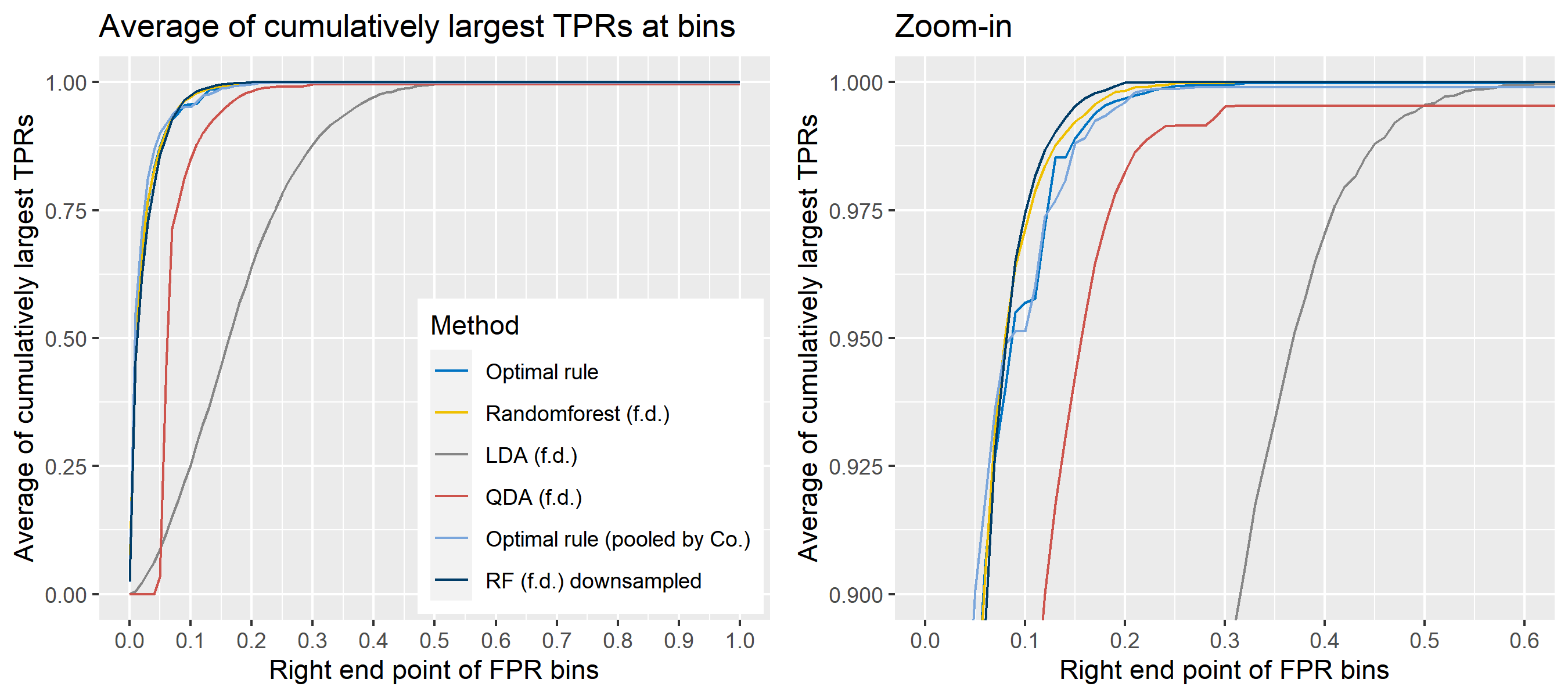
8.5.5.2 ROC curve for comparison
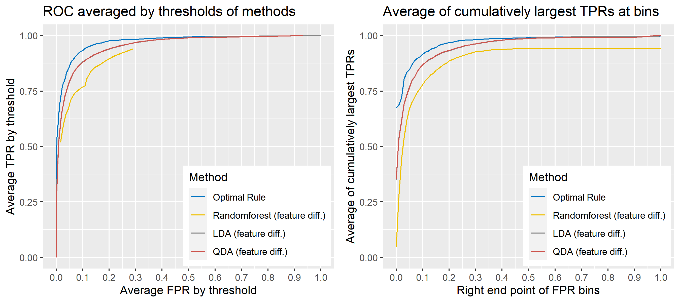
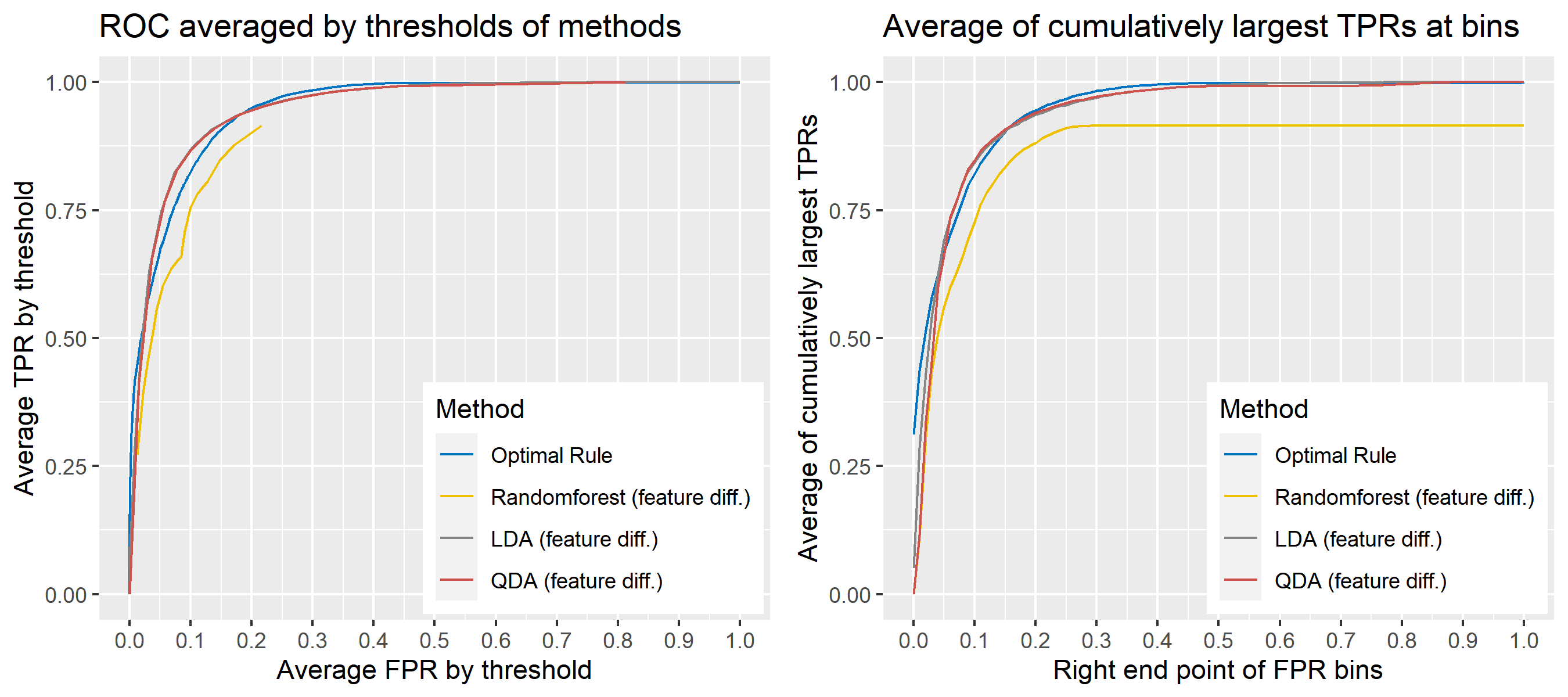
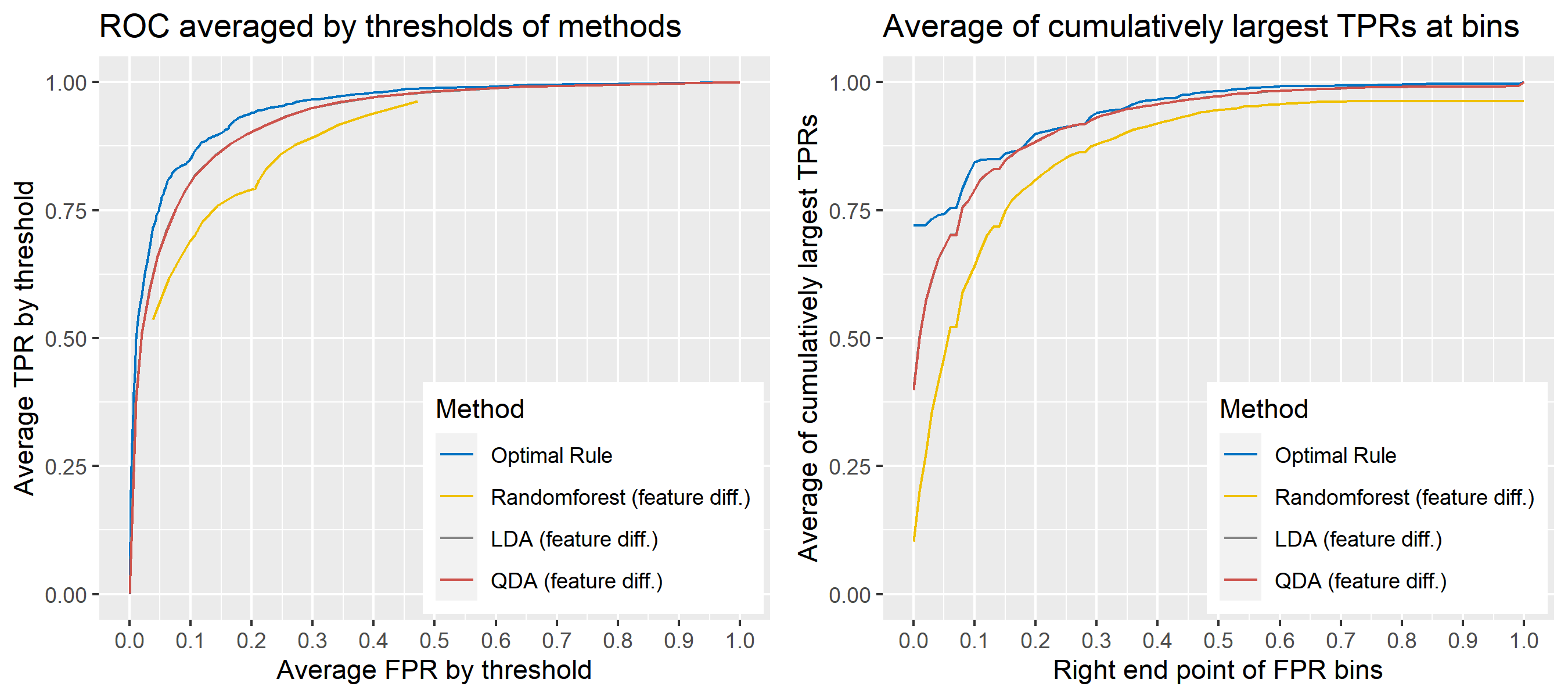
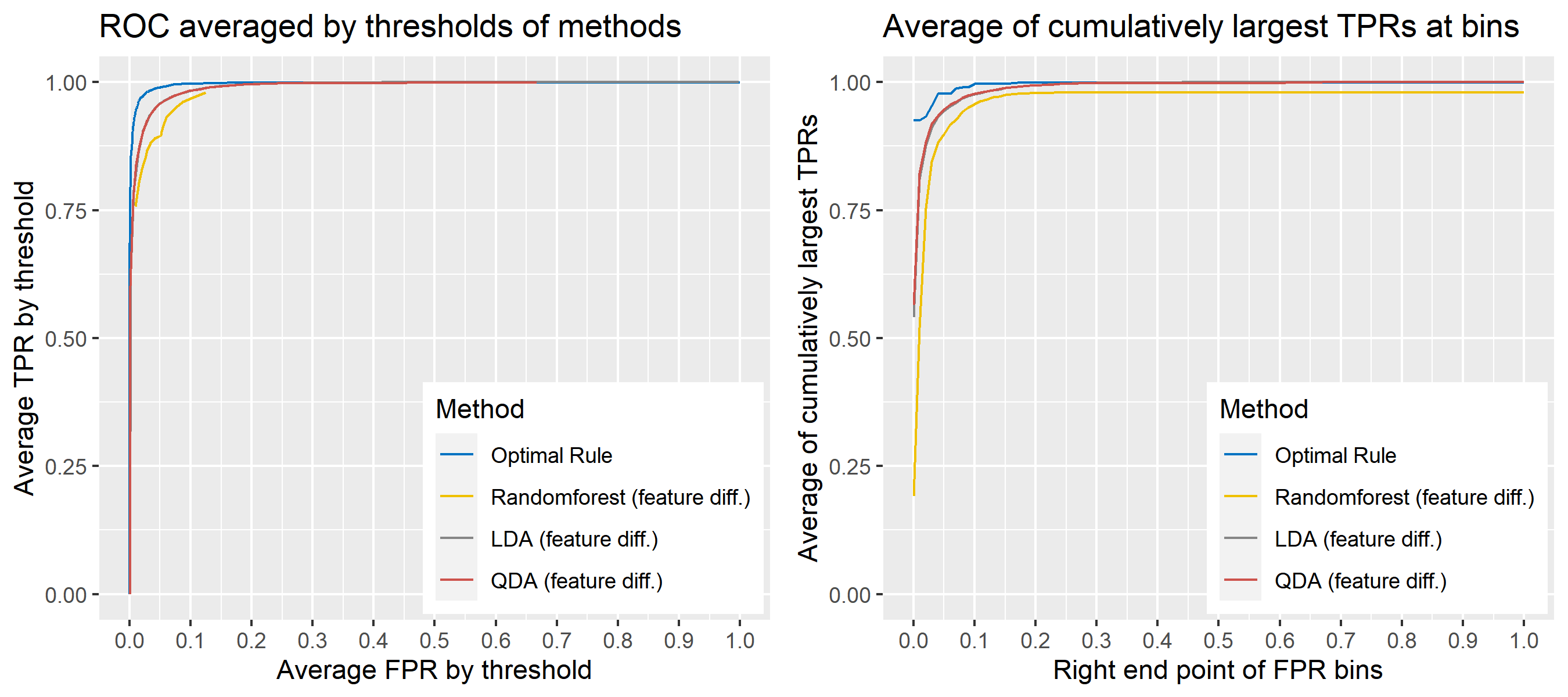
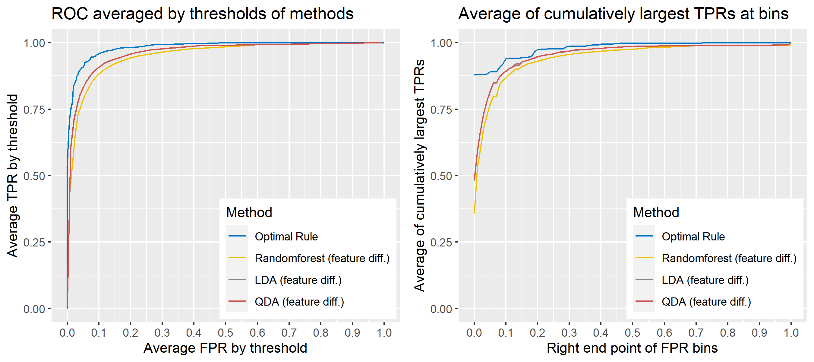
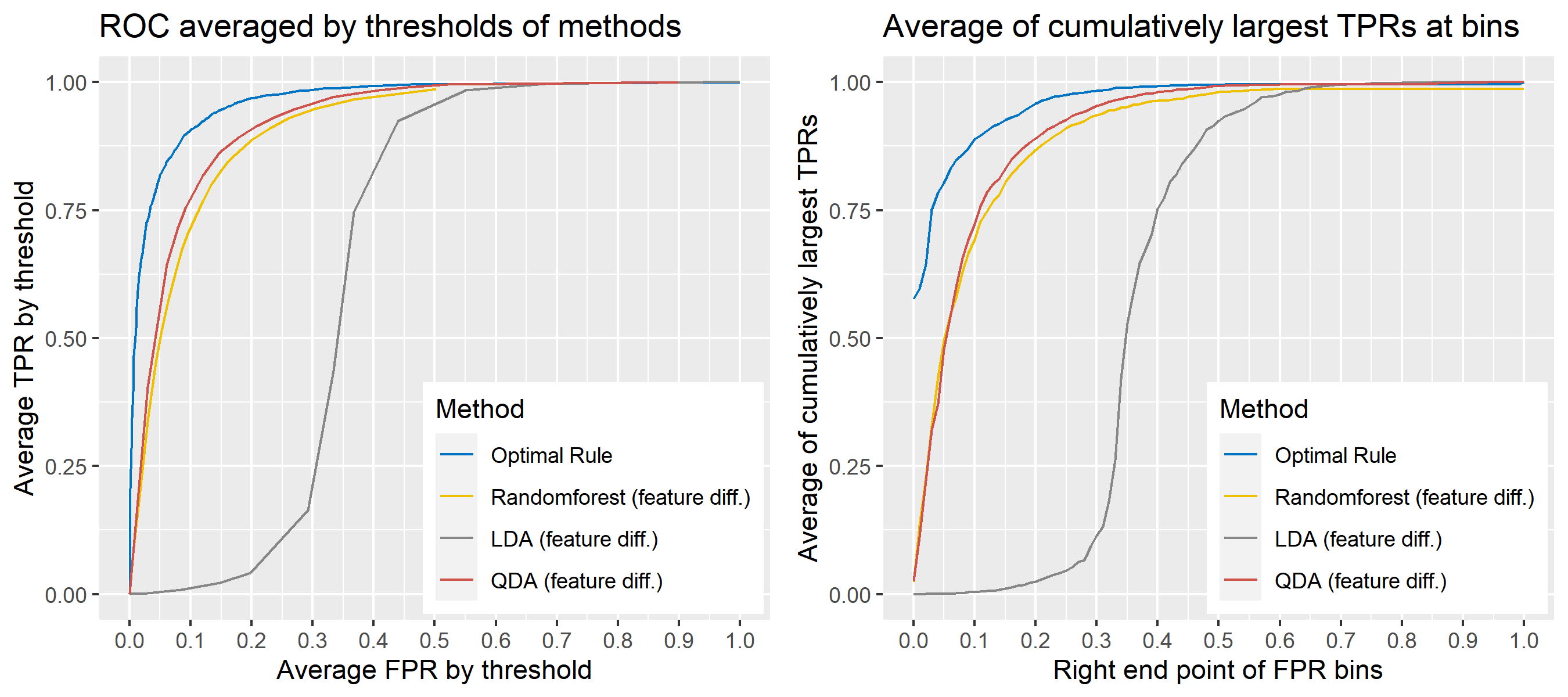
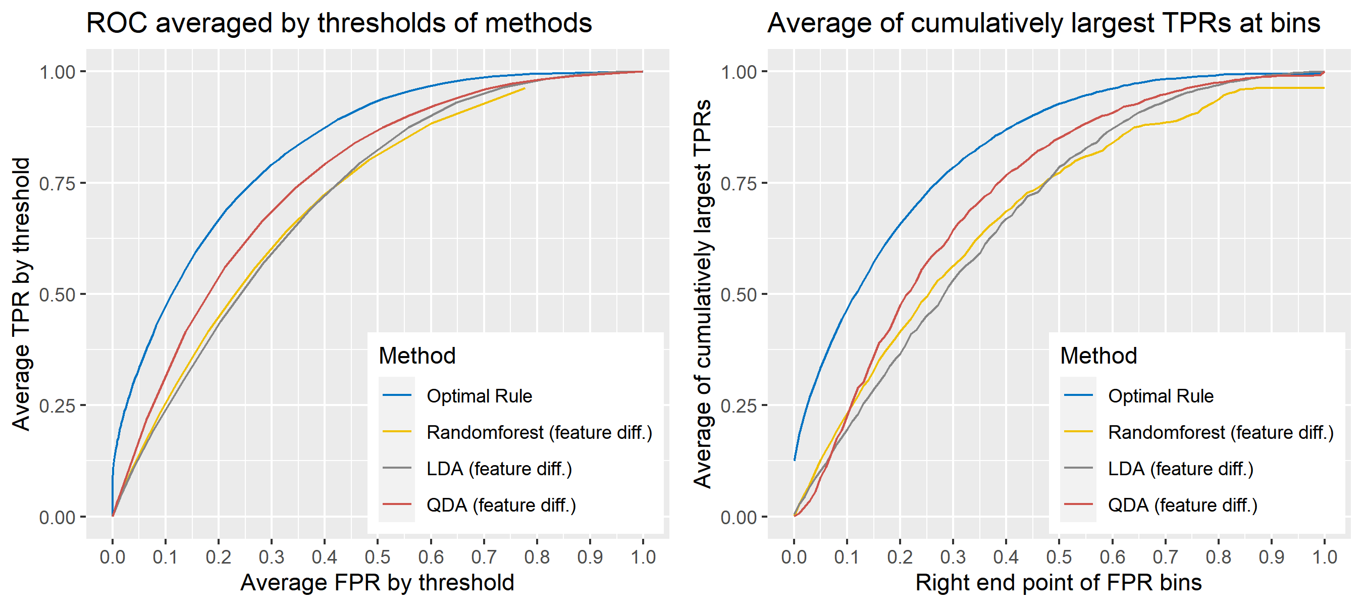
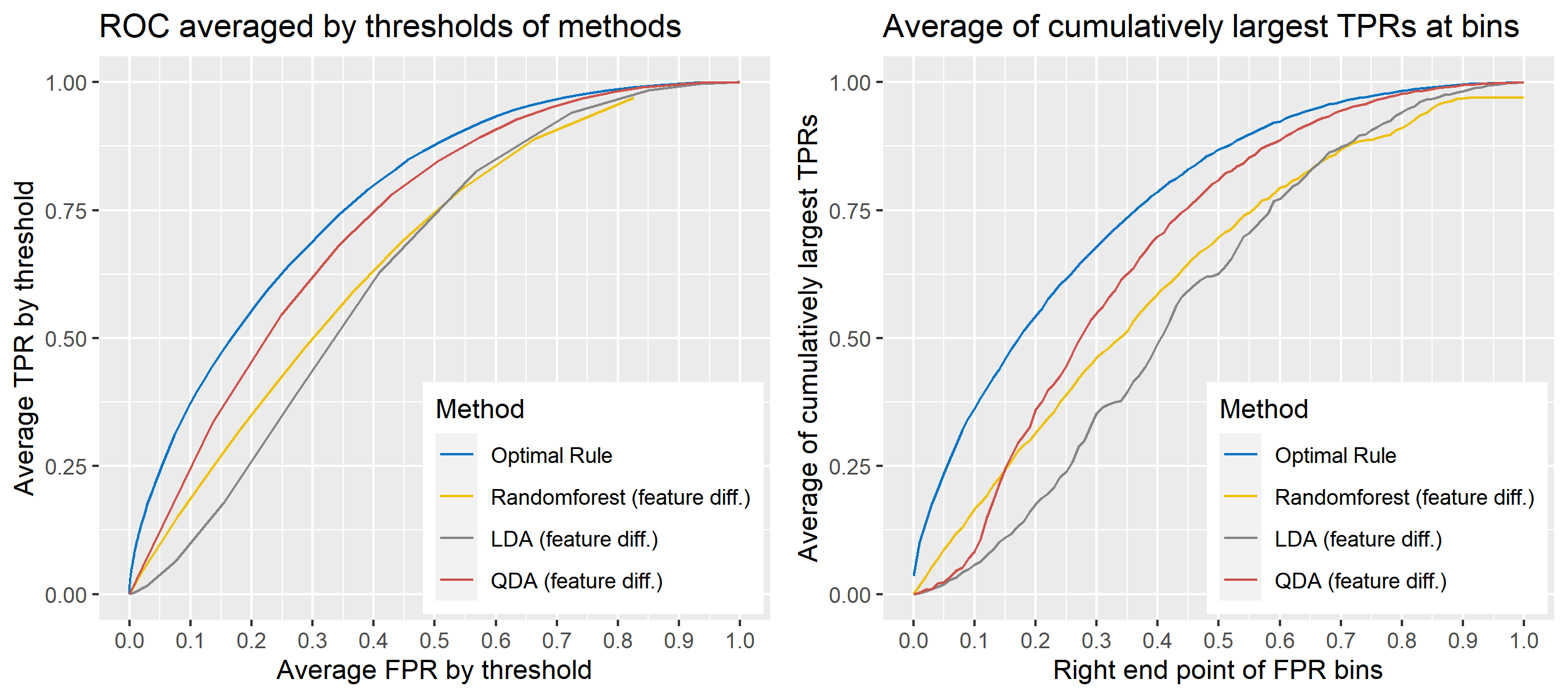
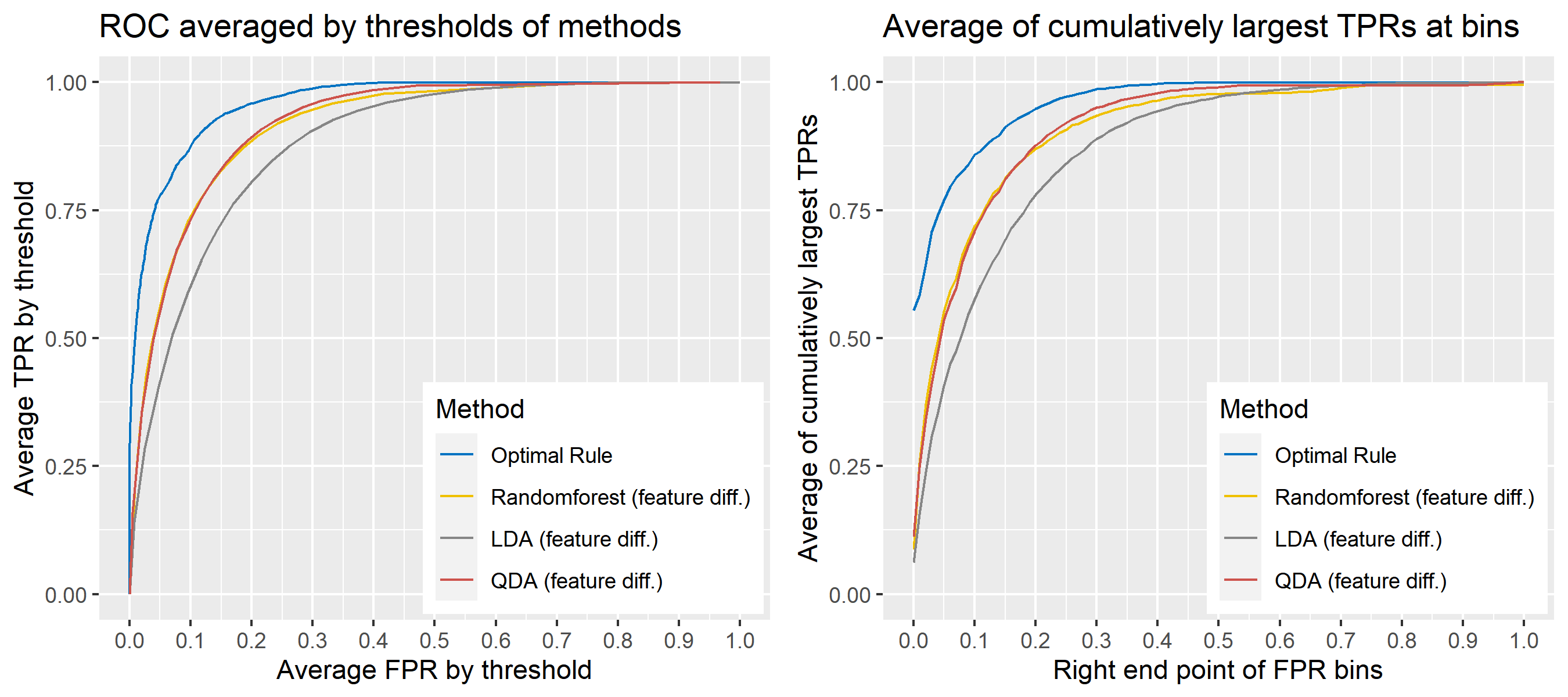
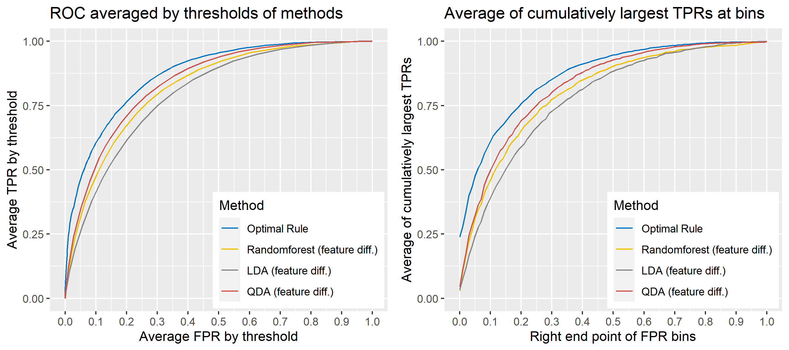
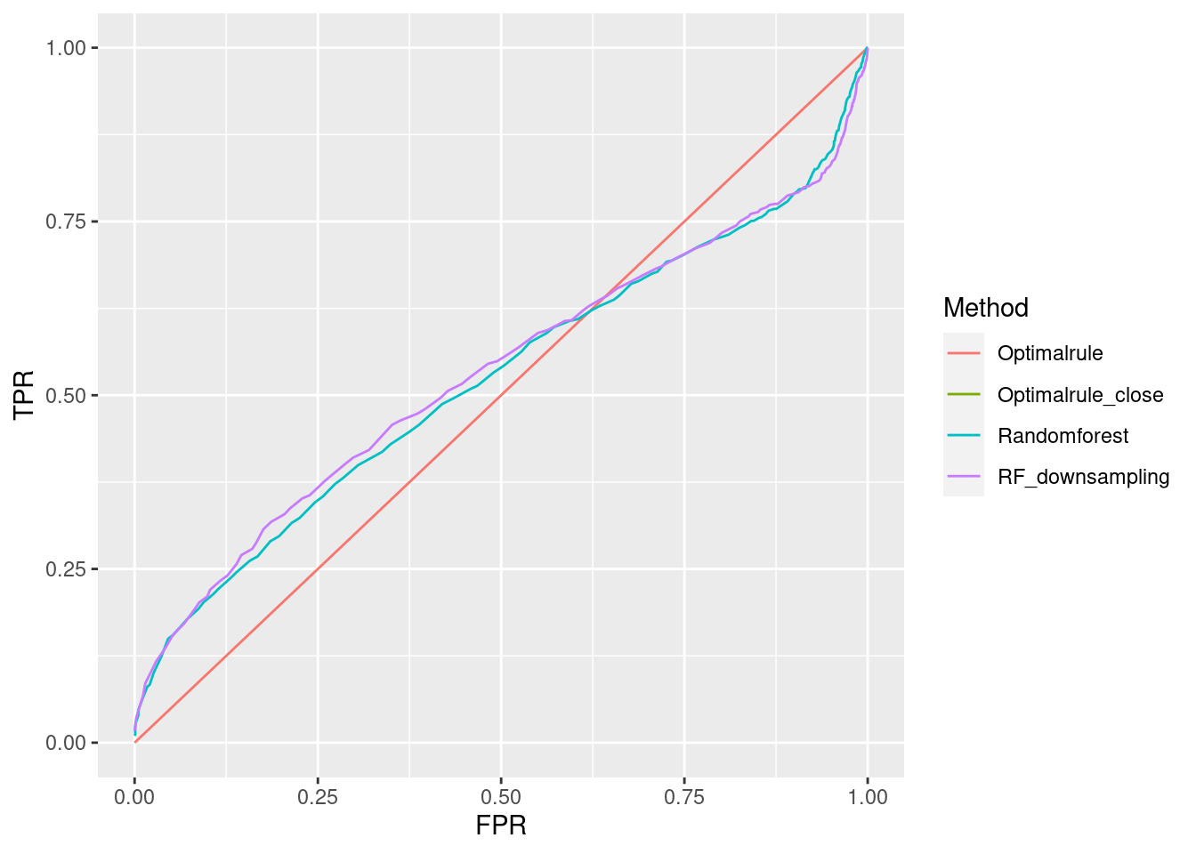
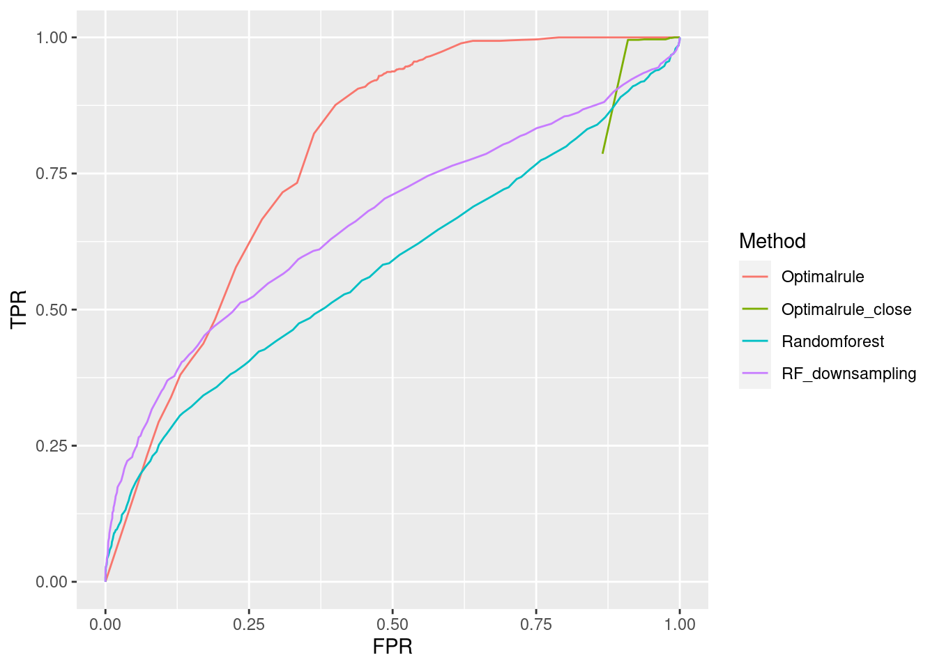
ROC curve is a diagnostic plot of binary classifiers, and with varying appropriate thresholds for a predictive model, ROC curve can be plotted, which is a great way to figure out predictive performance. The matching techniques we considered above are binary in that their prediction results for each pair of data represent whether the two observations are from the same sources or not rather than which source each observation would have come from. Thus, ROC curve will be used for comparing the matching techniques in this report.
Besides, threshold is different depending on matching methods, and varying threshold values lead to trade-off between true positive rate (TPR), and false positive rate (FPR). For optimal rule, the weight \(w\) in \(T_{SS}^{Opt, w}\) plays a role of threshold in ROC curve. We use prior probabilities as threshold for LDA and QDA based on feature differences where the prior indicates the probabilities of two groups—the same sources, and different sources—applied to the discriminant rules. Lastly, cutoff values for the two groups are used as threshold for randomforest so that the “winning” group for each pair of observations is the one with the maximum ratio of its vote share to cutoff.
8.5.5.3 Set-up for simulations
Assume that the conditional distribution, \(f(\cdot | \pi_g)\), is a normal distribution for any \(g = 1,\ \cdots,\ G\). The distributions will be used to generate data below. They may have different parameters for mean, variance, and covariance by a source, and some of them may share common parameters. For prior probabilities, \(p_g = 1/G\) is used so that the number of observations per a source is equal.
Step 1: According to the distributions for sources, 50 observations per a source are generated for a training set, and additional 10 observations per a source are generated for a test set. i.e., \(50 \times G\) observations in a training set and \(10 \times G\) observations in a test set.
Step 2: Pair all obesrvations in the test set. Hence, there will be the matching results for \({10G \choose 2}\) pairs in the test set so that whether the two observations in each pair would have come from the same sources or not are predicted.
Step 3: For a matching technique selected, using different thresholds, compute the false positive rate (FPR), and the true positive rate (TPR) based on the prediction results with the test set. Here, FPR indicates the estimated probability of the same source error and TPR indicates 1 minus the estimated probability of the different source error.
Step 4: By plotting the values of TPR over corresponding values of FPR, a single ROC curve is constructed.
Step 5: Repeat the step 1 to 4 100 times.
Step 6: Incorporate 100 ROC curves into a single monotonic ROC curve—e.g., incorporation by averaging out.
8.5.5.4 How to average multiple ROC curves
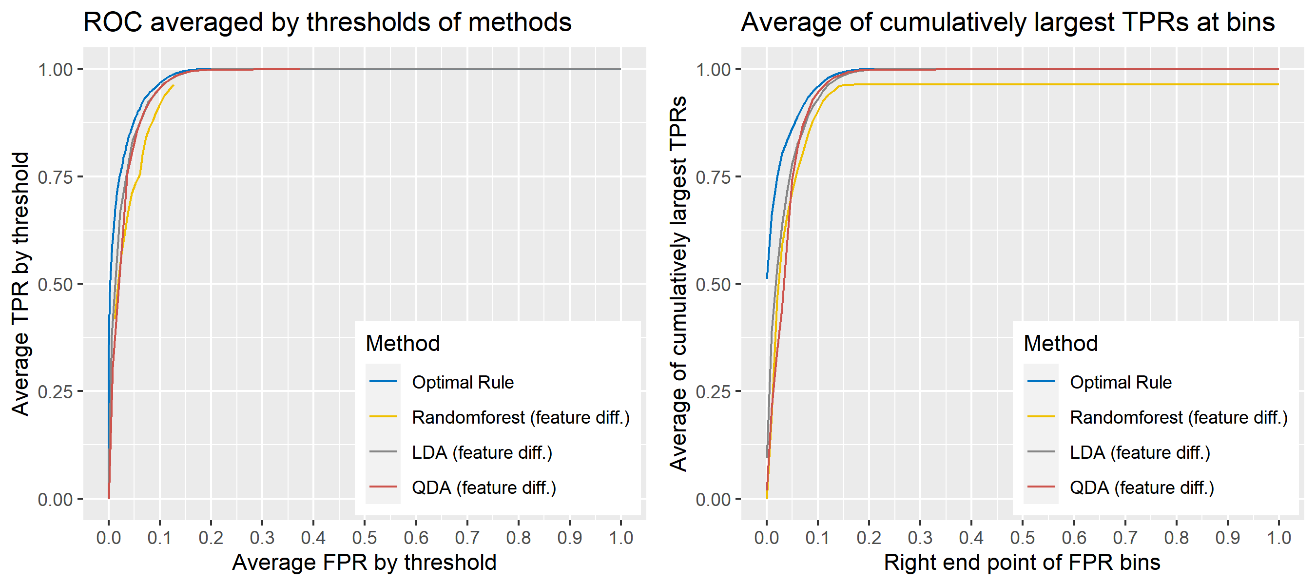
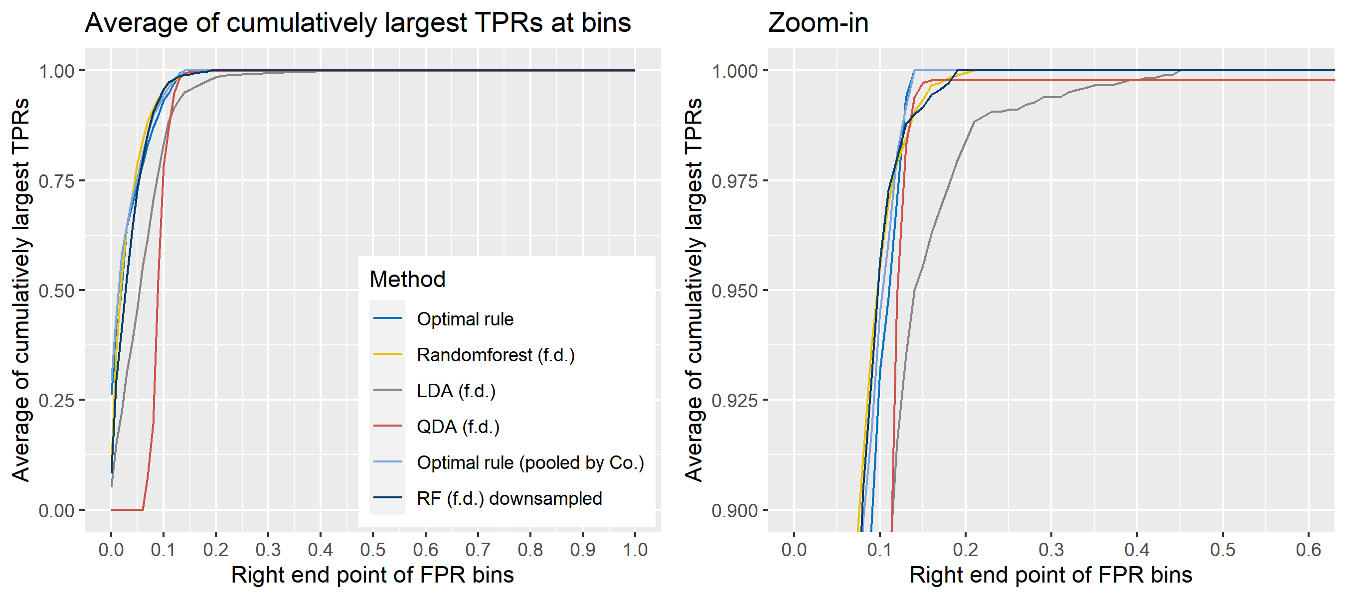
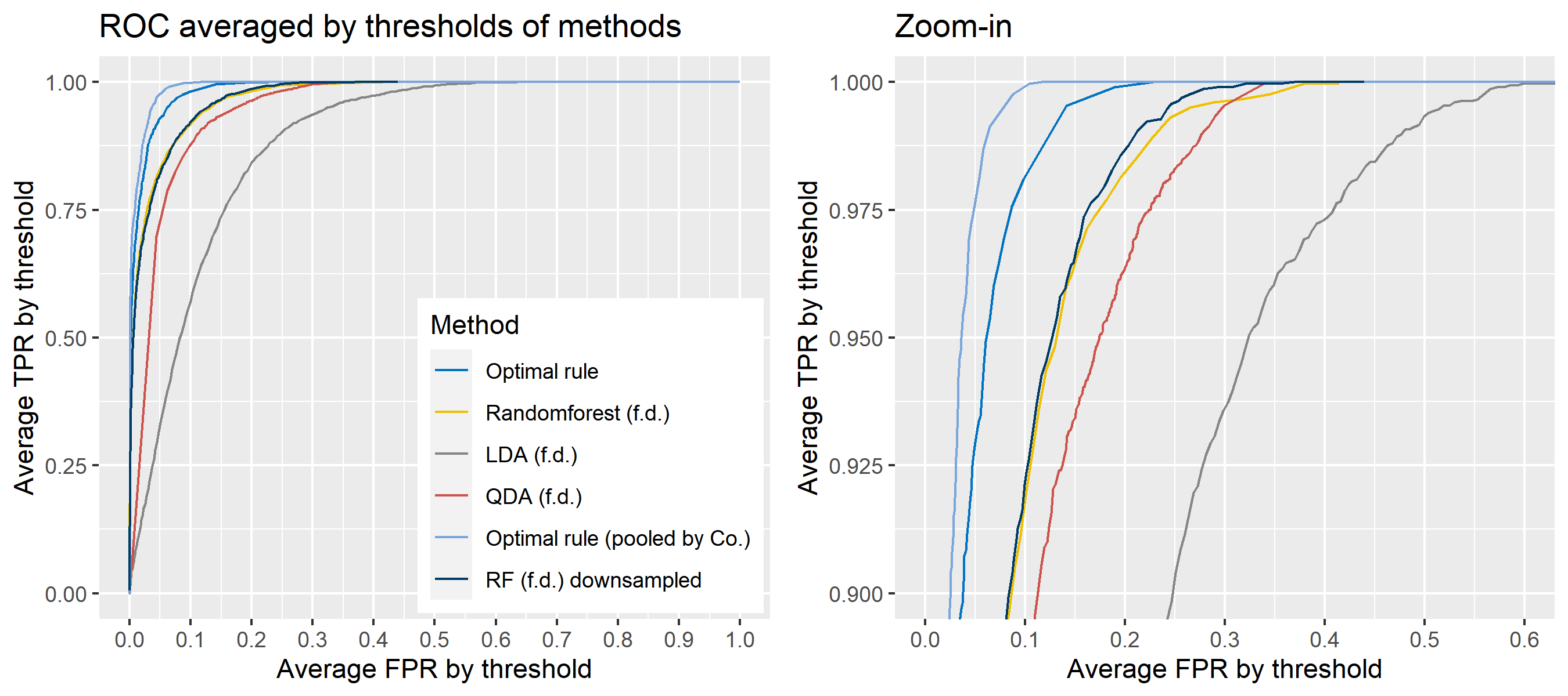
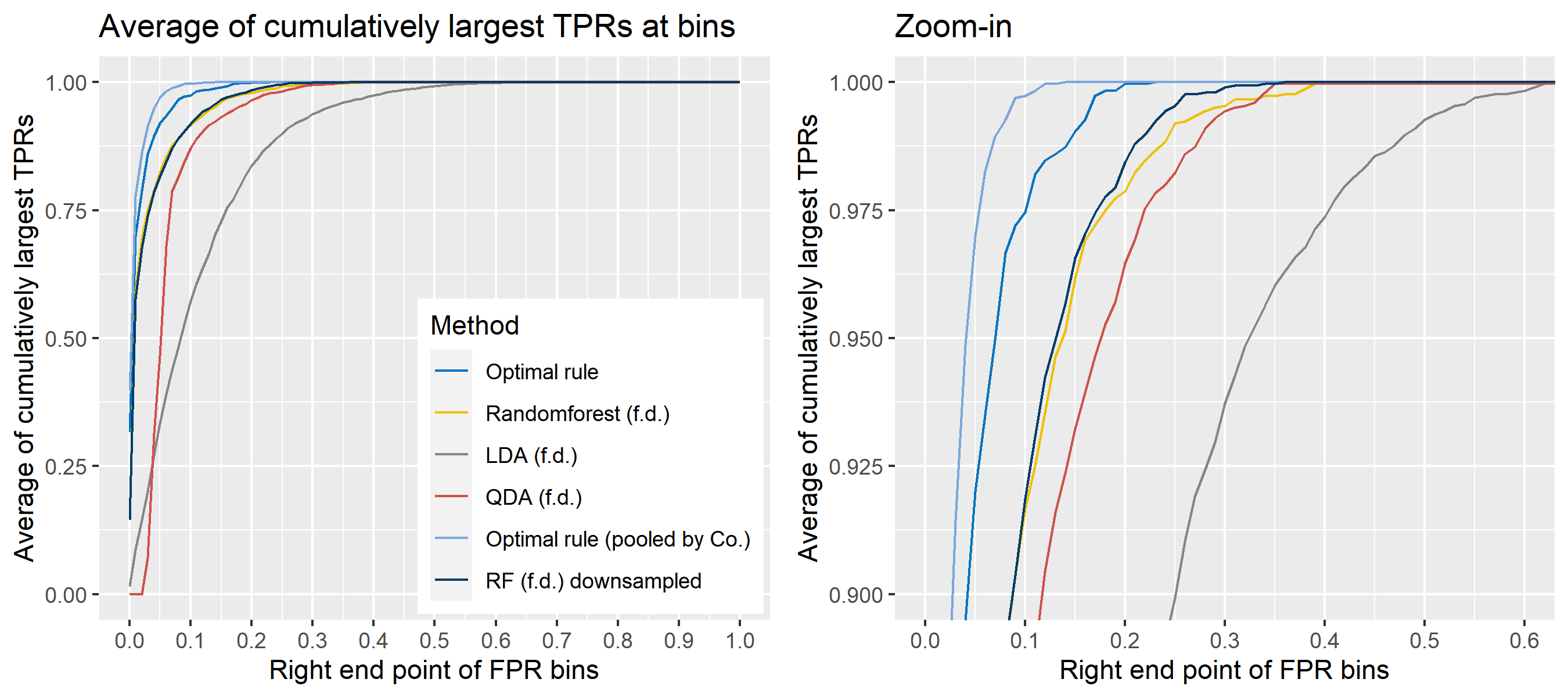
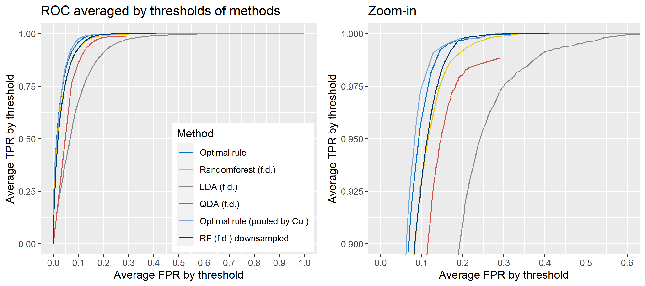
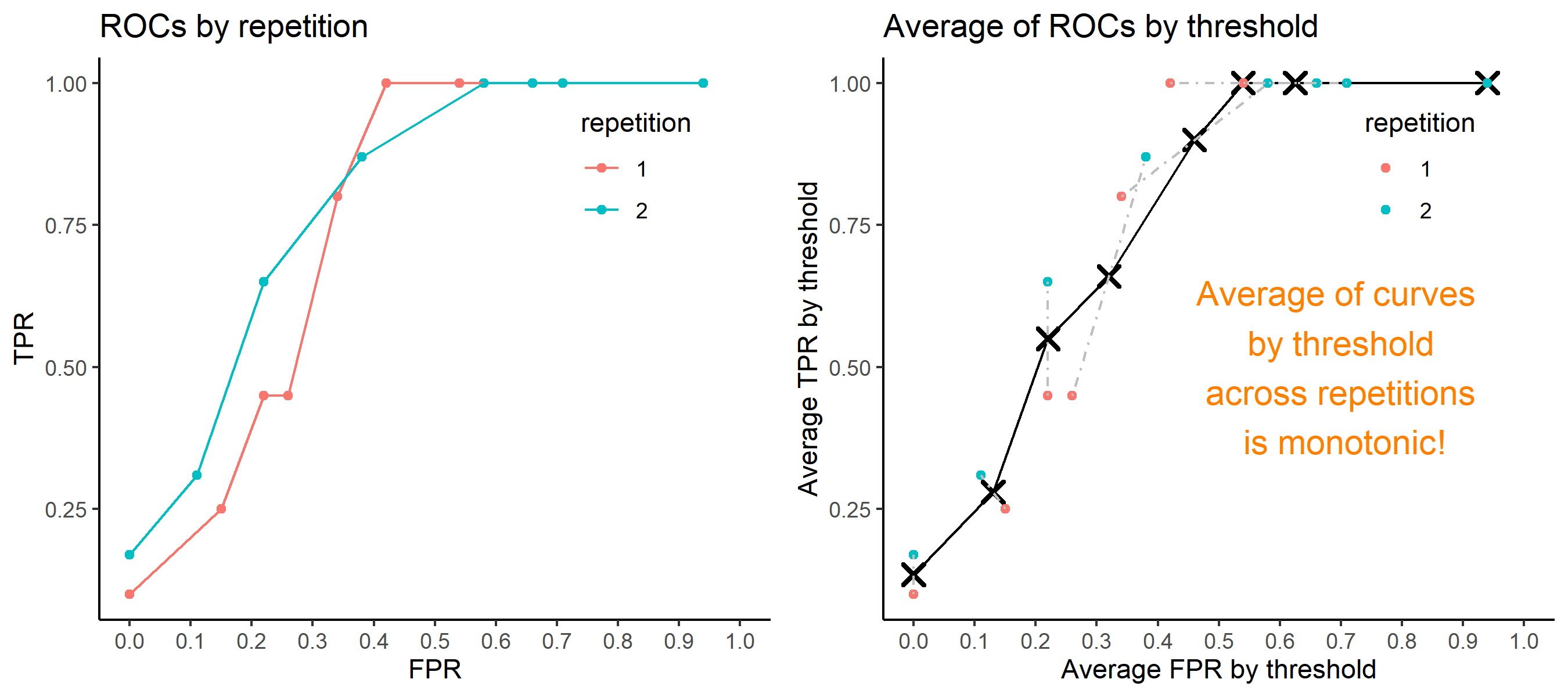
For the step 6, there are some issues of averaging multiple ROC curves by the values of FPR because no matter how densely the coordinates for (FPR, TPR) are formed, some ROC curves may not share common values of FPR. With that approach, the average ROC curve may be non-monotonic ROC curve which is not a desirable property of a ROC curve. The figure below illustrates the result.
Hence, we consider two differnt ways to average out, and the description and examples are shown below:
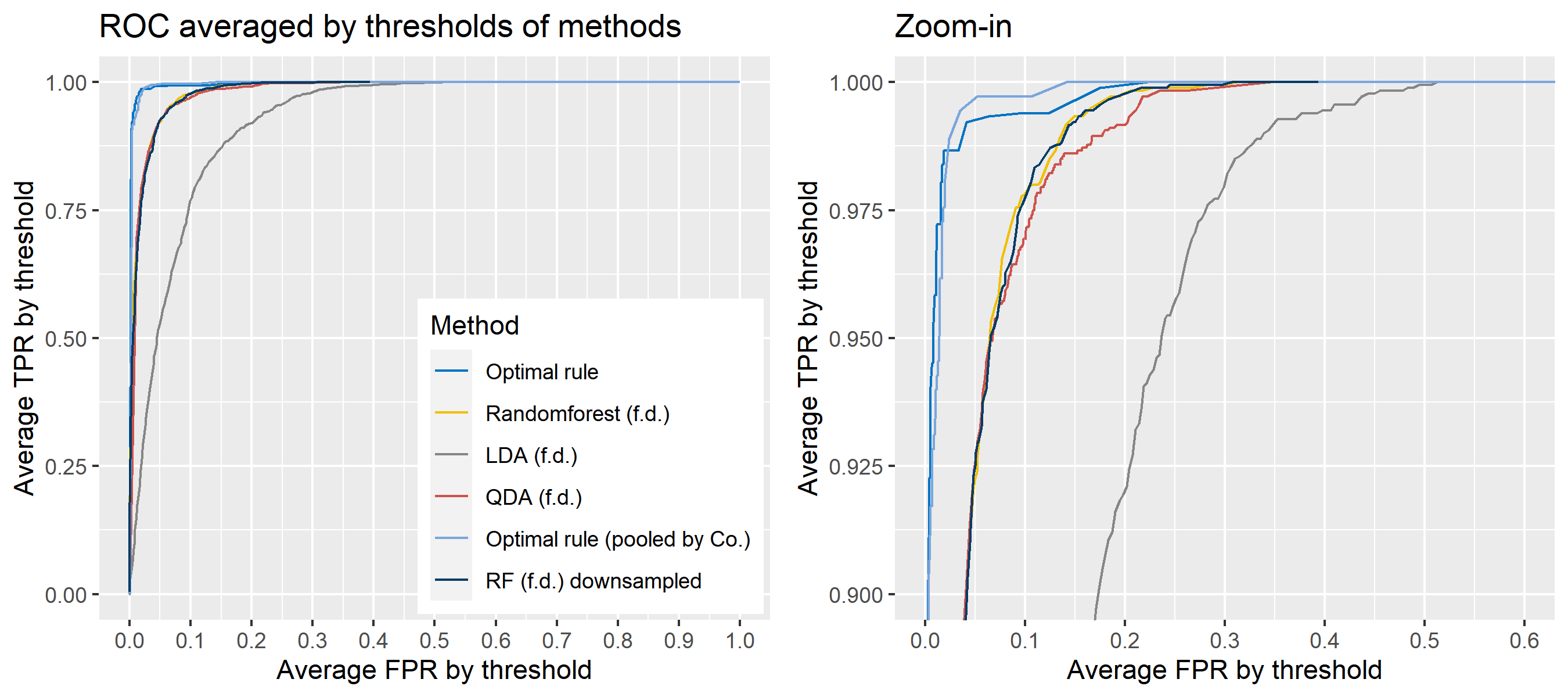
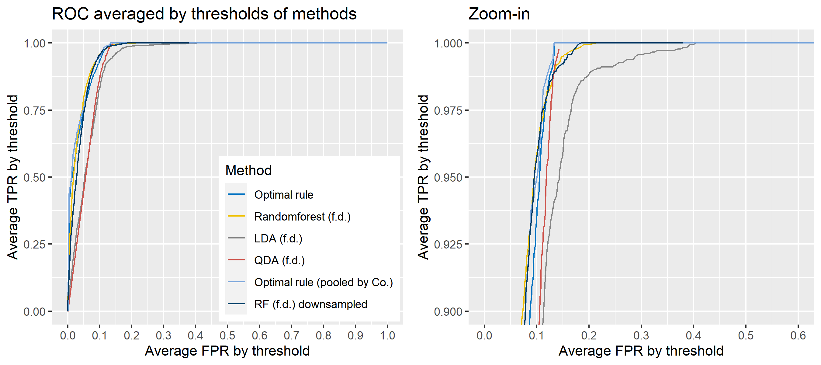
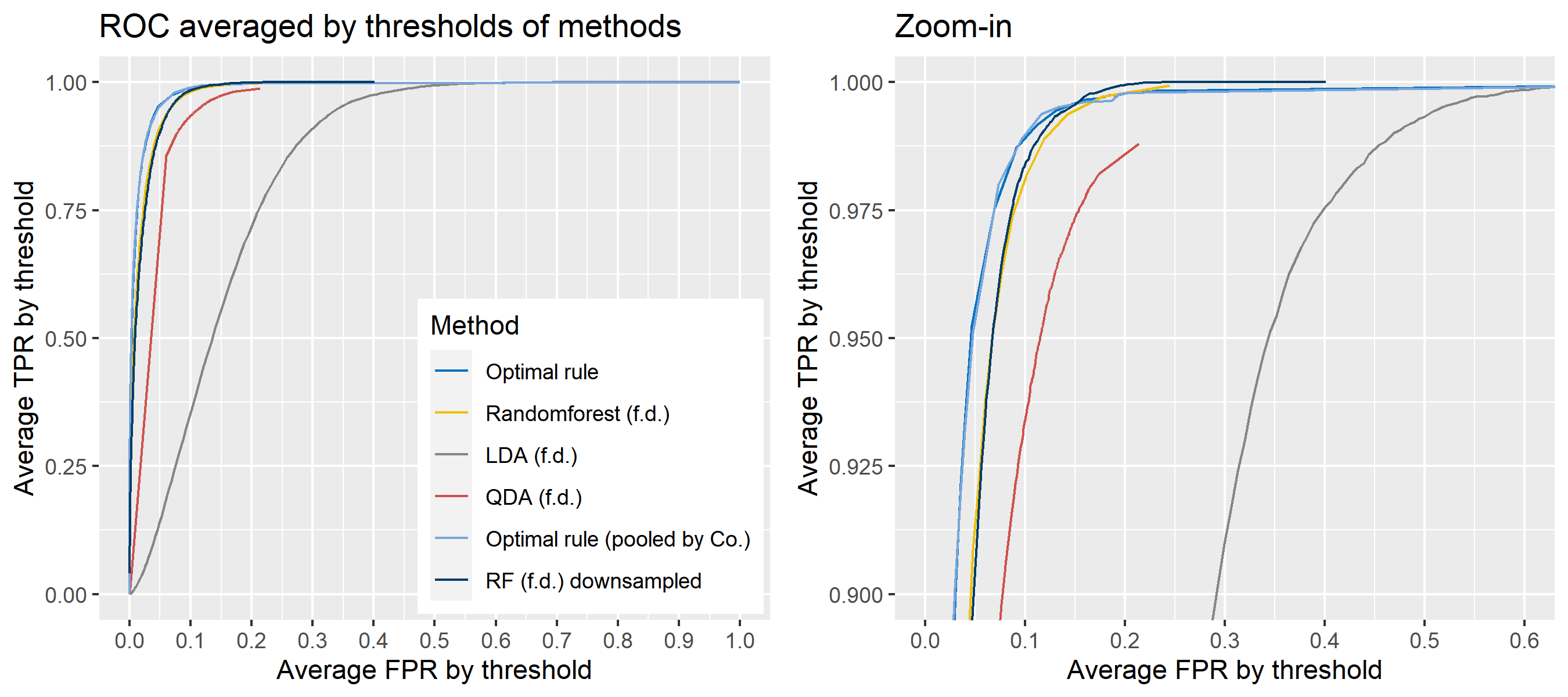
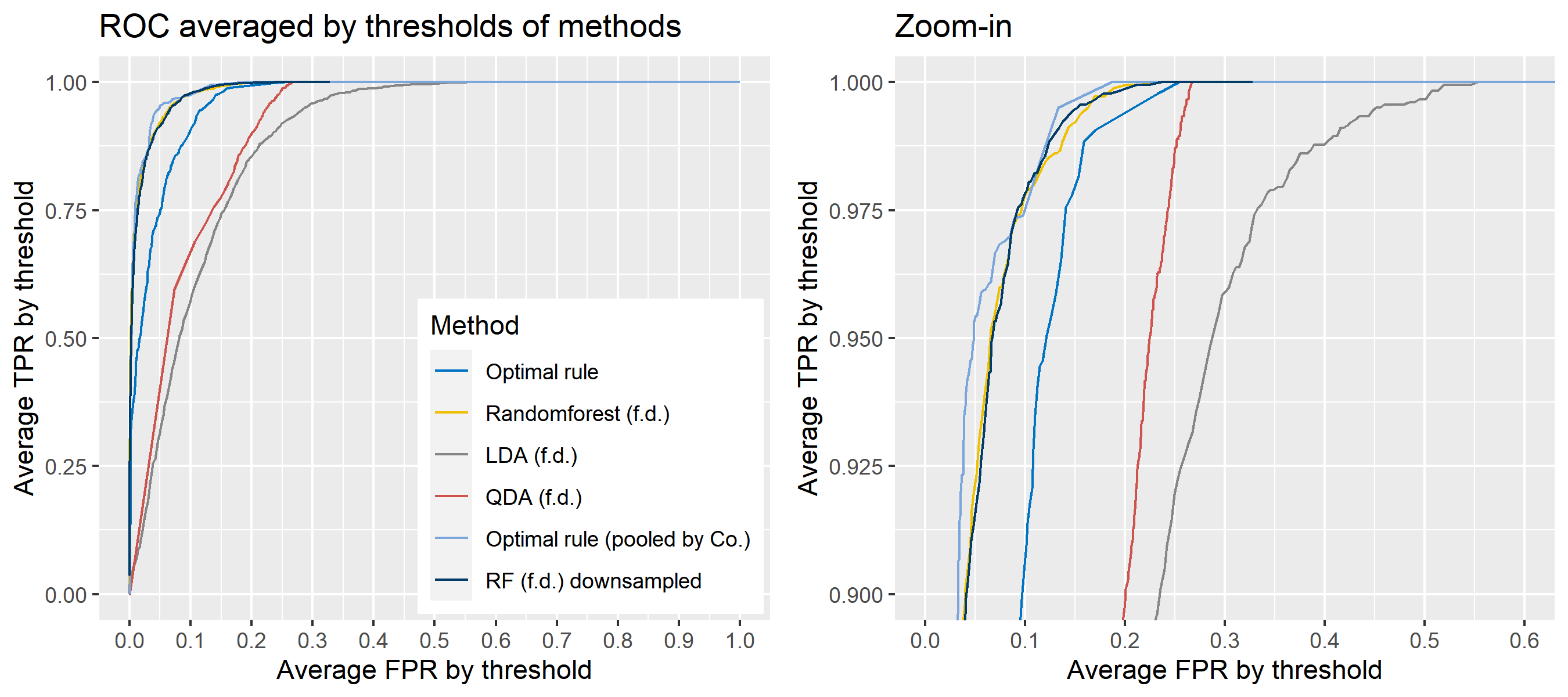
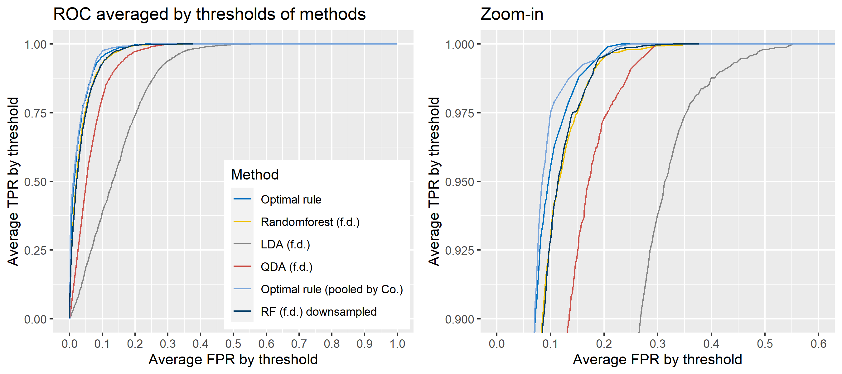
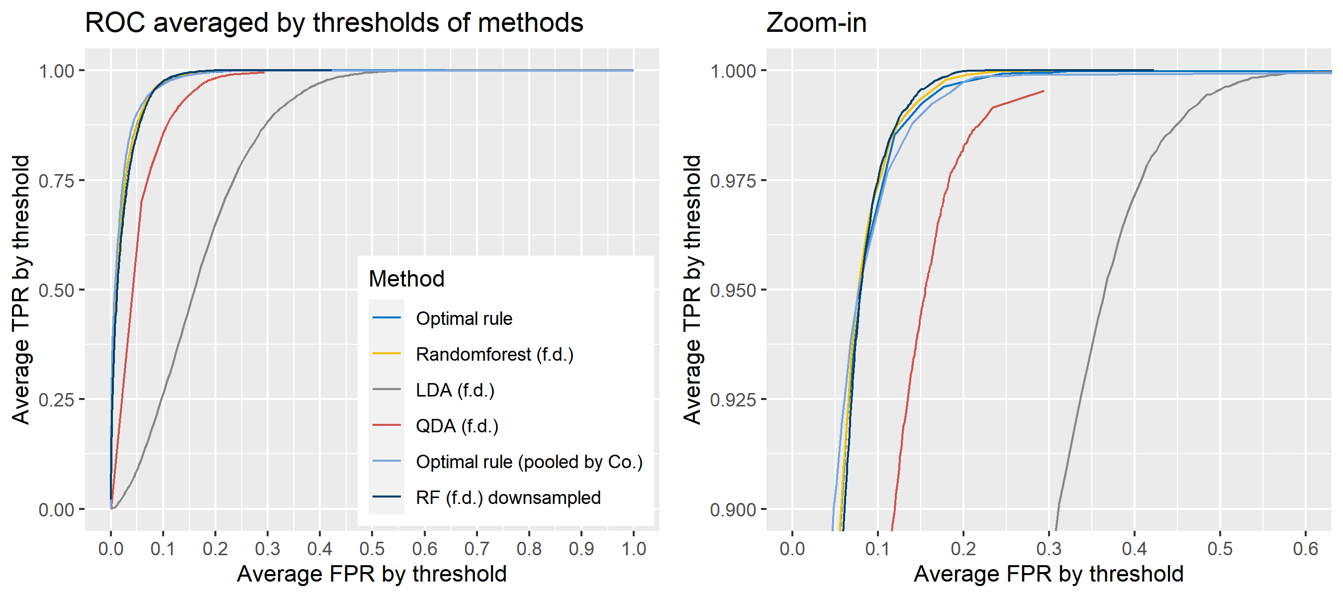
- Average of the values of TPRs and FPRs by threshold value
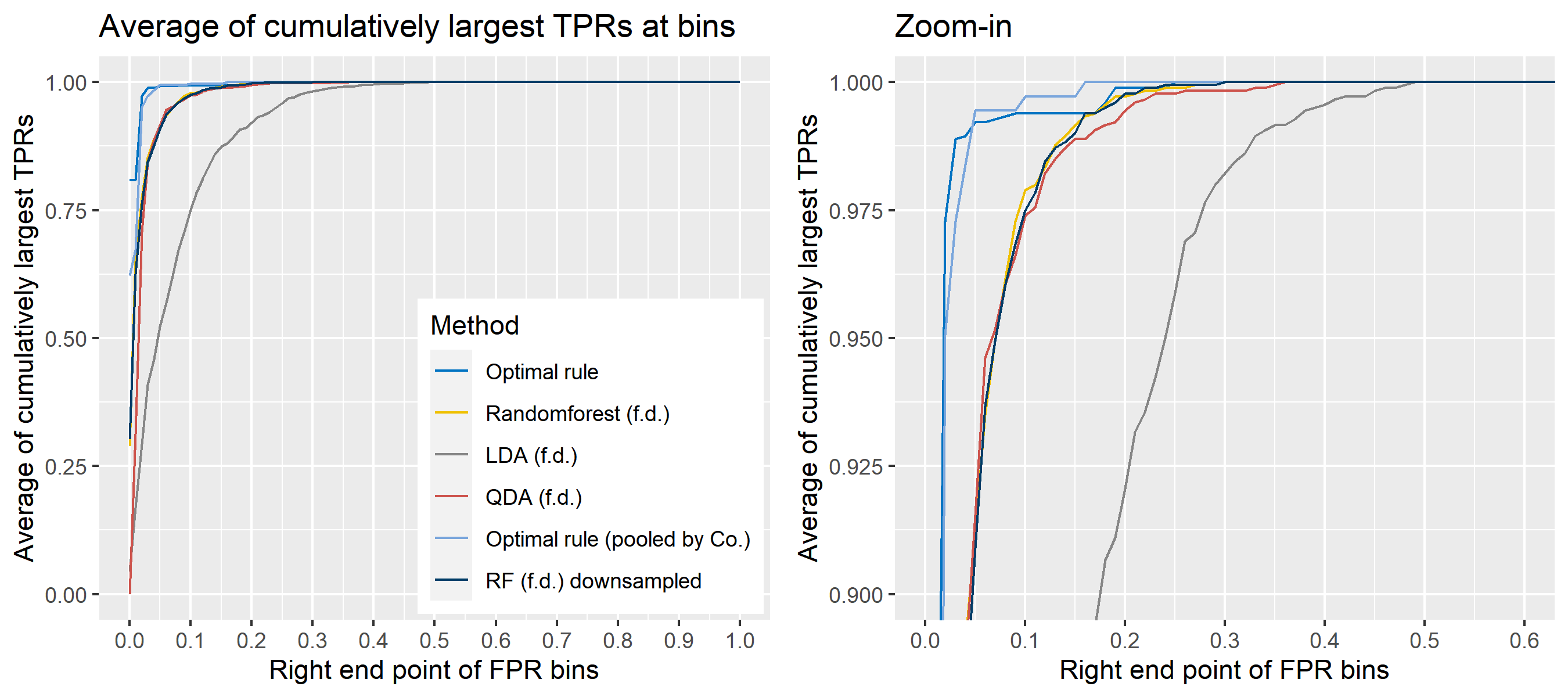
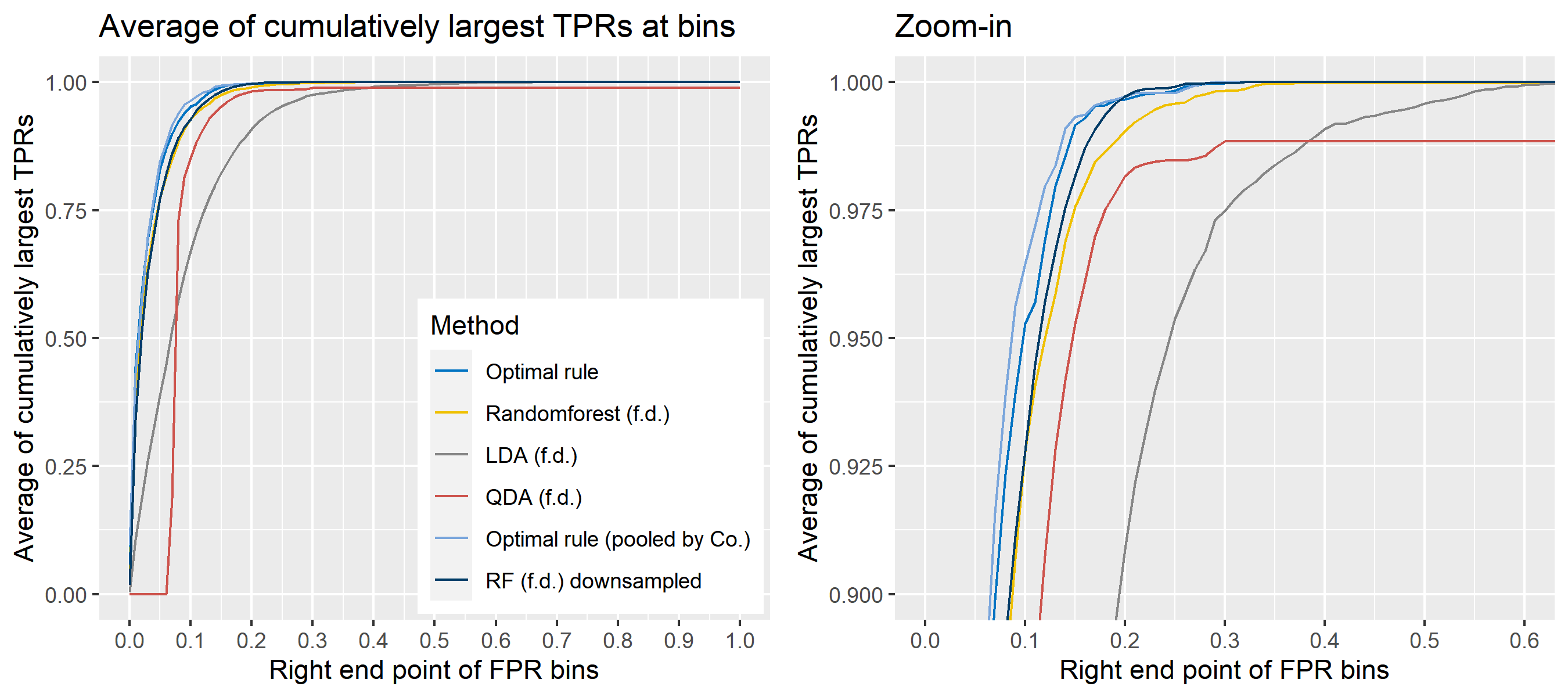
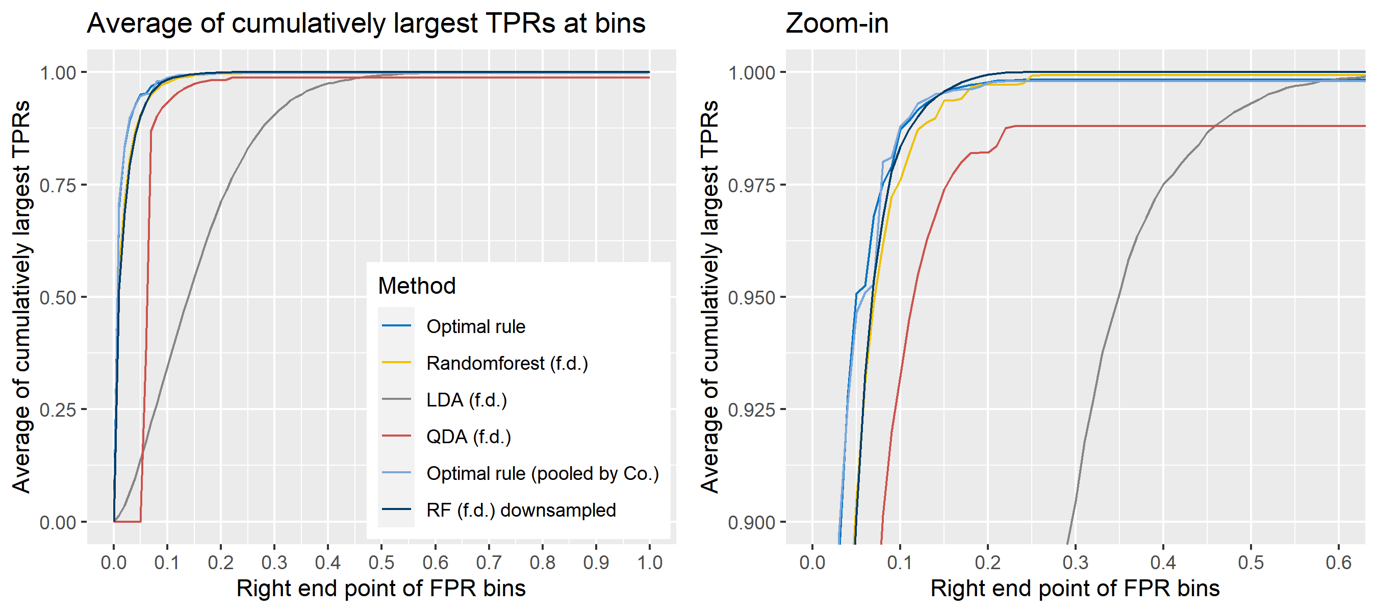
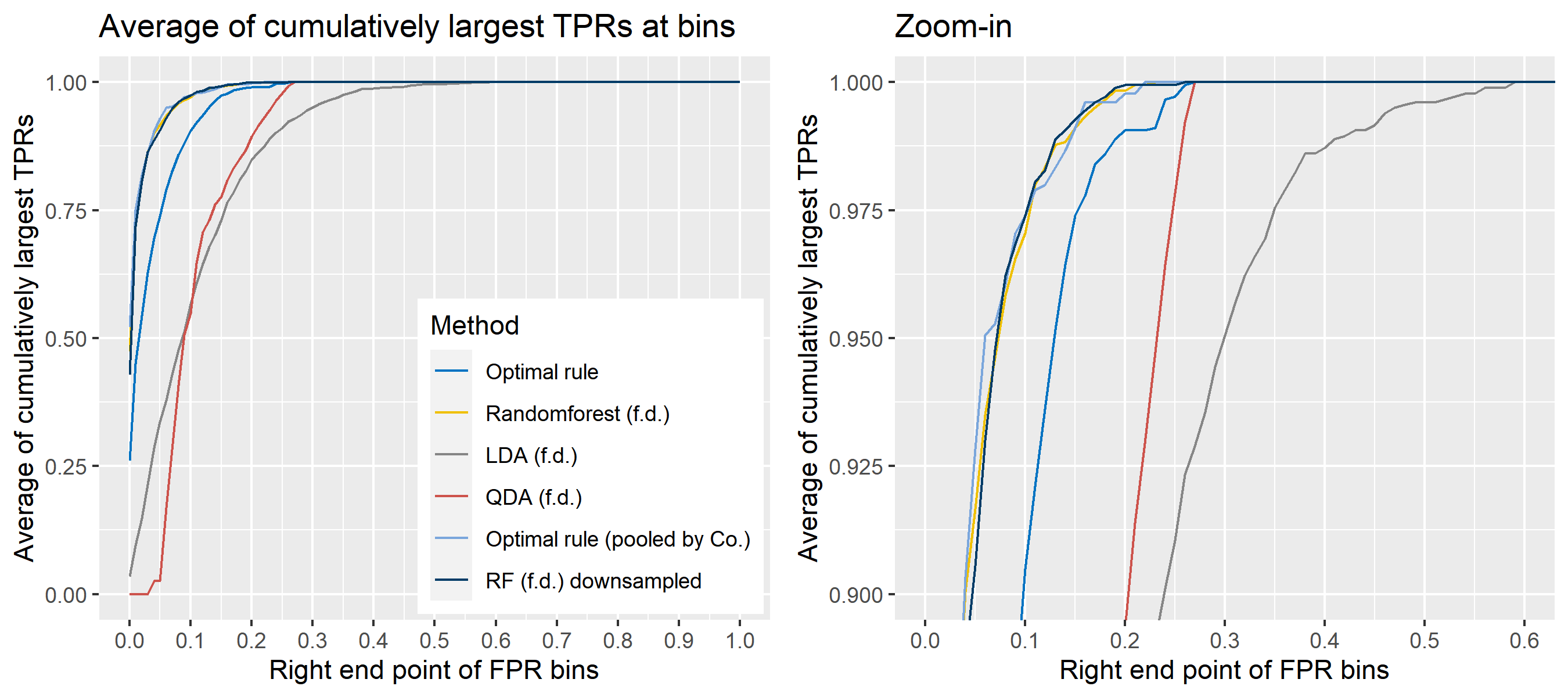
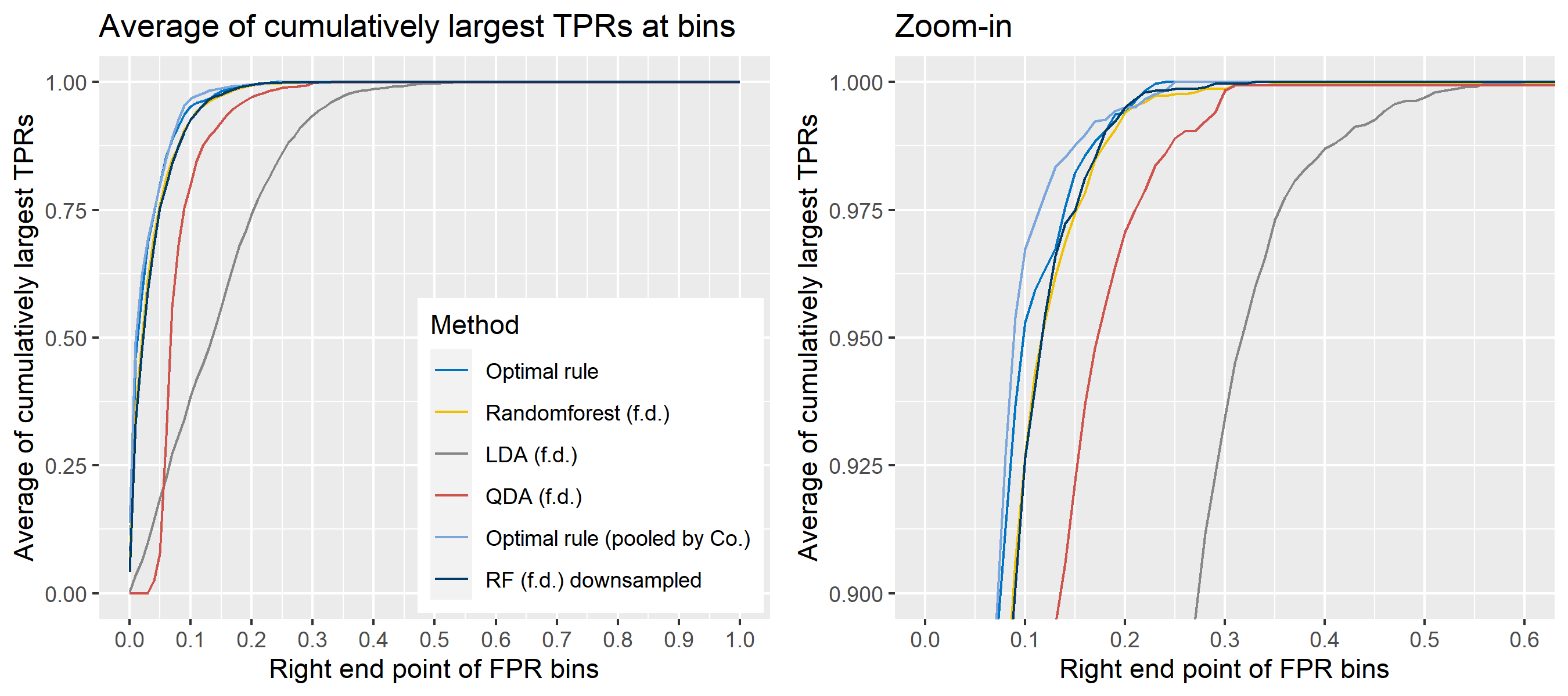
- Average of cumulatively largest vause of TPR in each bin for FPR.
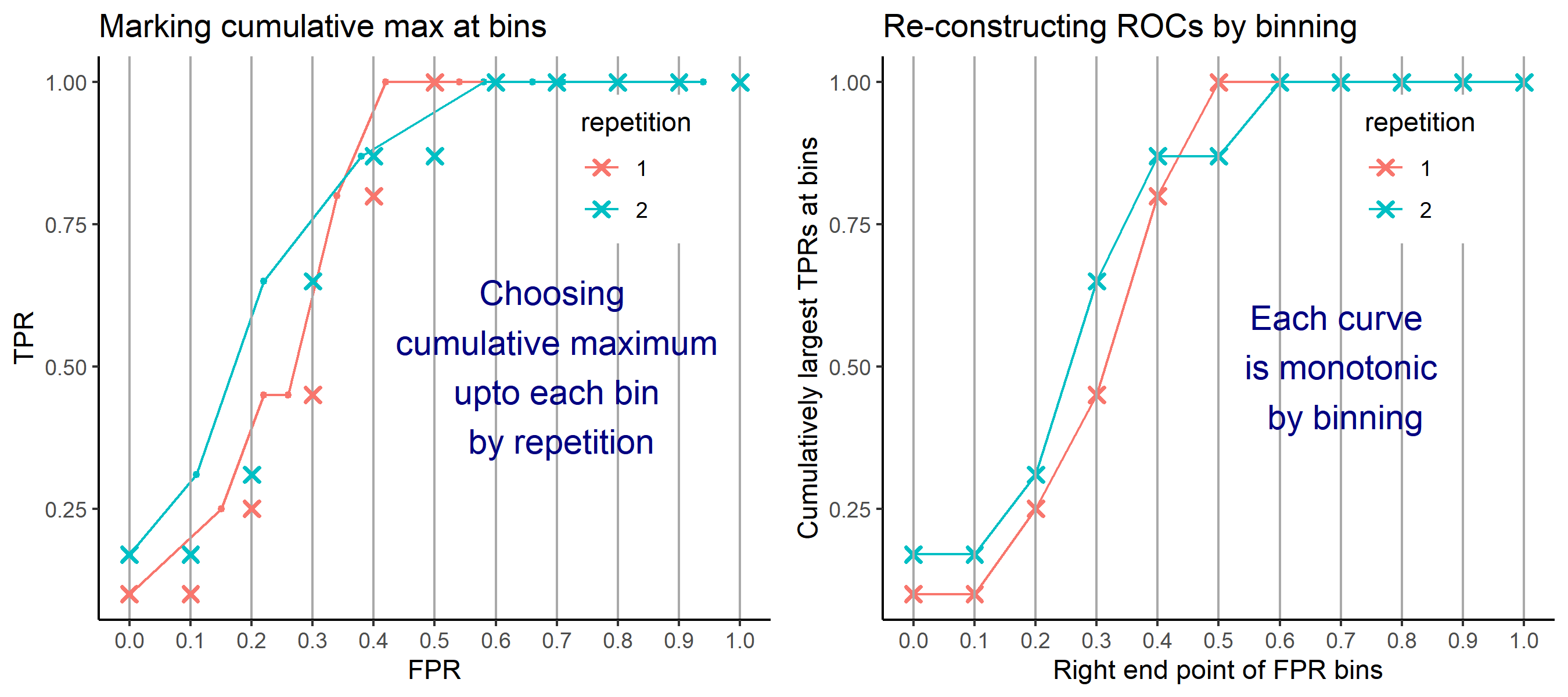
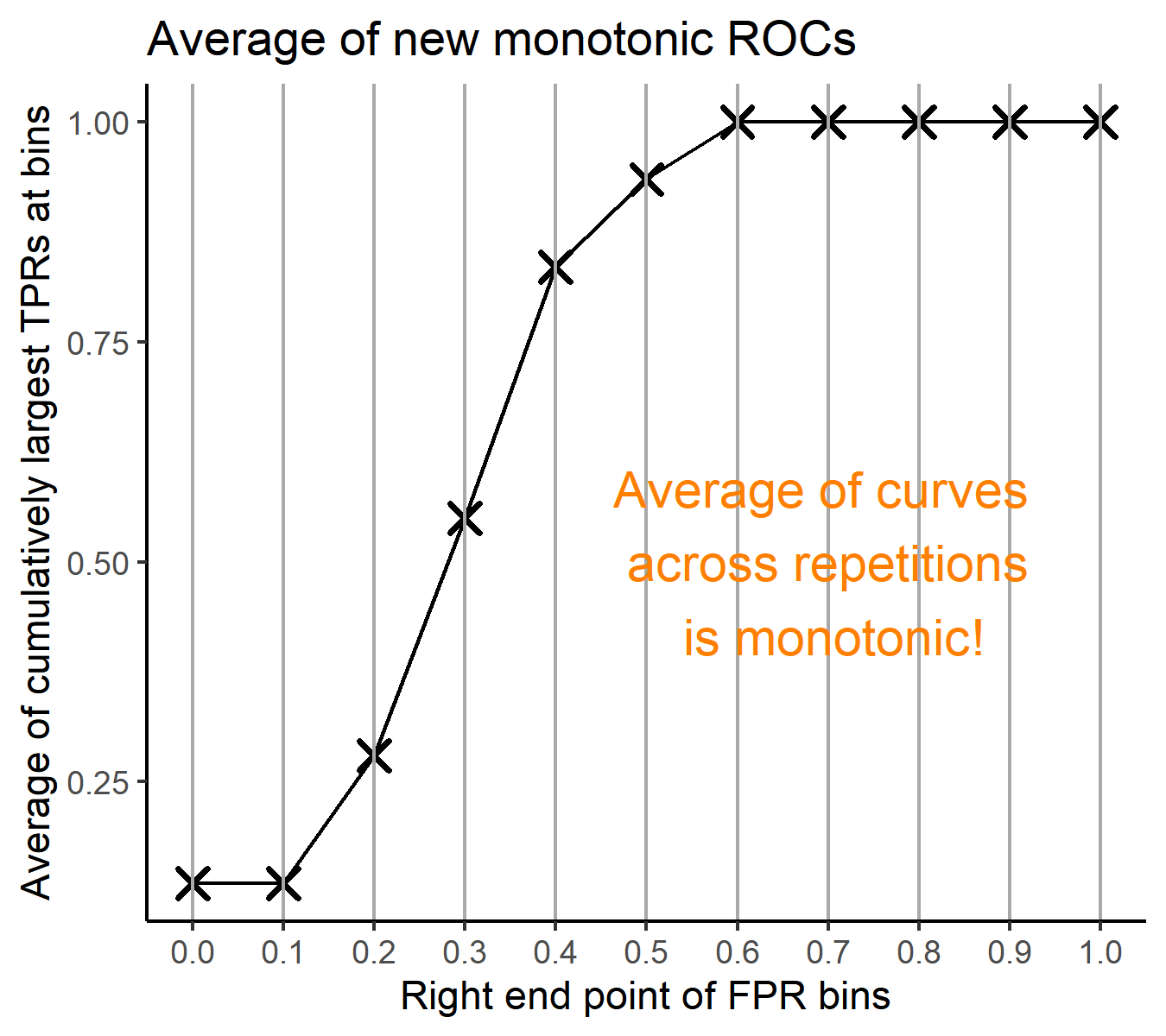
Like above, two types of average ROC curves will be provided for comparing the performance of several methods.
8.5.6 Simulation results
8.5.6.1 Univariate Result 1
## Warning: `vec_depth()` was deprecated in purrr 1.0.0.
## ℹ Please use `pluck_depth()` instead.
## This warning is displayed once every 8 hours.
## Call `lifecycle::last_lifecycle_warnings()` to see where this warning was
## generated.
## Error in loadNamespace(x): there is no package called 'rlist'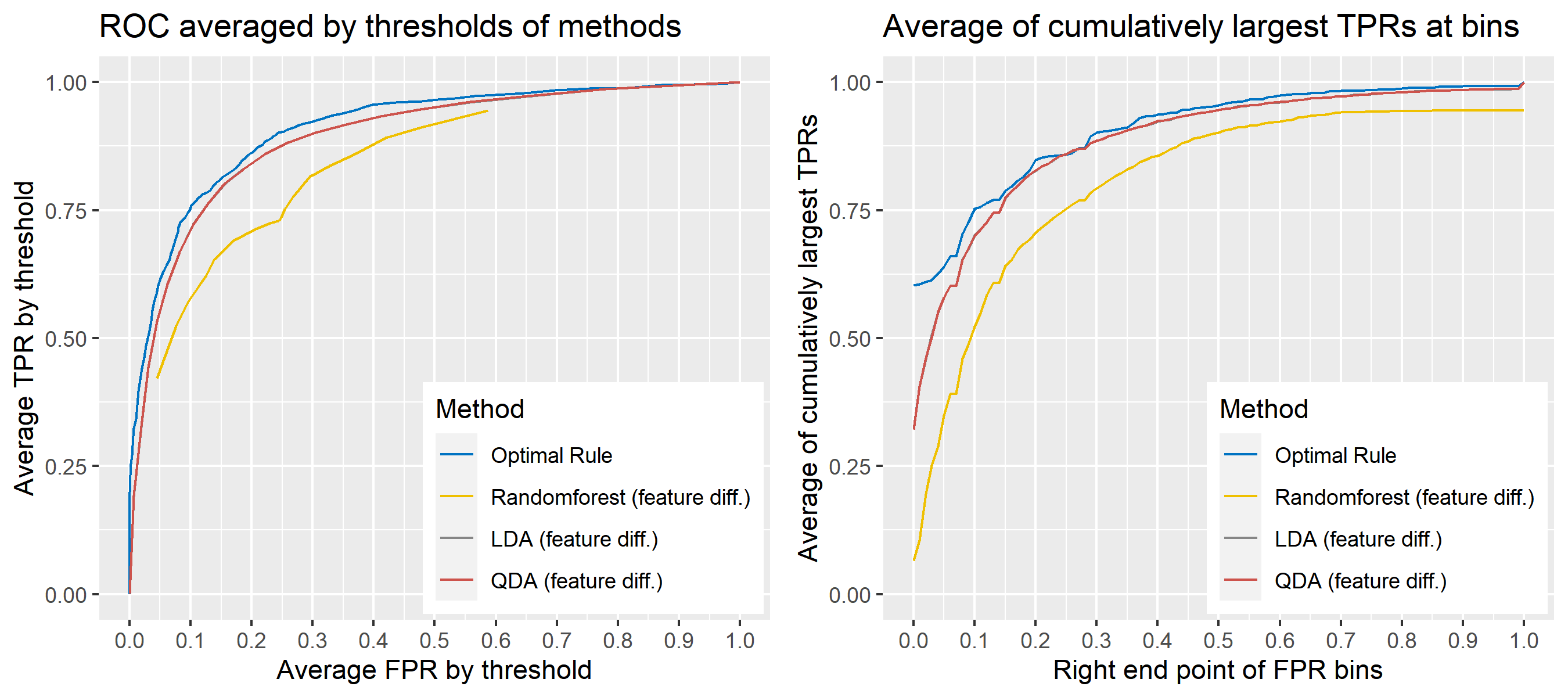
8.5.6.7 Multivariate Result 1; G = 2, N = 2
| \[\mbox{Source, }g\] | \[\mu_g\] | \[\Sigma_g\] |
|---|---|---|
| \[1\] | \[\begin{bmatrix} 10&-10 \end{bmatrix}'\] | \[\begin{bmatrix} 16&-4\\-4&25 \end{bmatrix}\] |
| \[2\] | \[\begin{bmatrix} -1&1 \end{bmatrix}'\] | \[\begin{bmatrix} 9&4\\4&36 \end{bmatrix}\] |
8.5.6.8 Multivariate Result 2
| \[\mbox{Source, }g\] | \[\mu_g\] | \[\Sigma_g\] |
|---|---|---|
| \[1\] | \[\begin{bmatrix} 10&-10 \end{bmatrix}'\] | \[\begin{bmatrix} 16&-4\\-4&25 \end{bmatrix}\] |
| \[2\] | \[\begin{bmatrix} -1&1 \end{bmatrix}'\] | \[\begin{bmatrix} 9&4\\4&36 \end{bmatrix}\] |
| \[3\] | \[\begin{bmatrix} 20&-20 \end{bmatrix}'\] | \[\begin{bmatrix} 16&-9\\-9&25 \end{bmatrix}\] |
8.5.6.9 Multivariate Result 3
| \[\mbox{Source, }g\] | \[\mu_g\] | \[\Sigma_g\] |
|---|---|---|
| \[1\] | \[\begin{bmatrix} 1&10 \end{bmatrix}'\] | \[\begin{bmatrix} 1&-1\\-1&4 \end{bmatrix}\] |
| \[2\] | \[\begin{bmatrix} -1&12 \end{bmatrix}'\] | \[\begin{bmatrix} 1&0.5\\0.5&1 \end{bmatrix}\] |
| \[3\] | \[\begin{bmatrix} 0&10 \end{bmatrix}'\] | \[\begin{bmatrix} 1&-1.5\\-1.5&4 \end{bmatrix}\] |
| \[4\] | \[\begin{bmatrix} 2&8 \end{bmatrix}'\] | \[\begin{bmatrix} 1&-0.1\\-0.1&4 \end{bmatrix}\] |
| \[5\] | \[\begin{bmatrix} -2&7 \end{bmatrix}'\] | \[\begin{bmatrix} 4&-2\\-2&4 \end{bmatrix}\] |
8.5.6.10 Multivariate Result 4
| \[\mbox{Source, }g\] | \[\mu_g\] | \[\Sigma_g\] |
|---|---|---|
| \[1\] | \[\begin{bmatrix} 3&10&5 \end{bmatrix}'\] | \[\begin{bmatrix} 4&2&-0.3\\2&25&8\\-0.3&8&9 \end{bmatrix}\] |
| \[2\] | \[\begin{bmatrix} -1&20&15 \end{bmatrix}'\] | \[\begin{bmatrix} 4&2&-3\\2&49&2\\-3&2&9 \end{bmatrix}\] |
| \[3\] | \[\begin{bmatrix} -5&30&25 \end{bmatrix}'\] | \[\begin{bmatrix} 4&1&-0.3\\1&36&1\\-0.3&1&9 \end{bmatrix}\] |
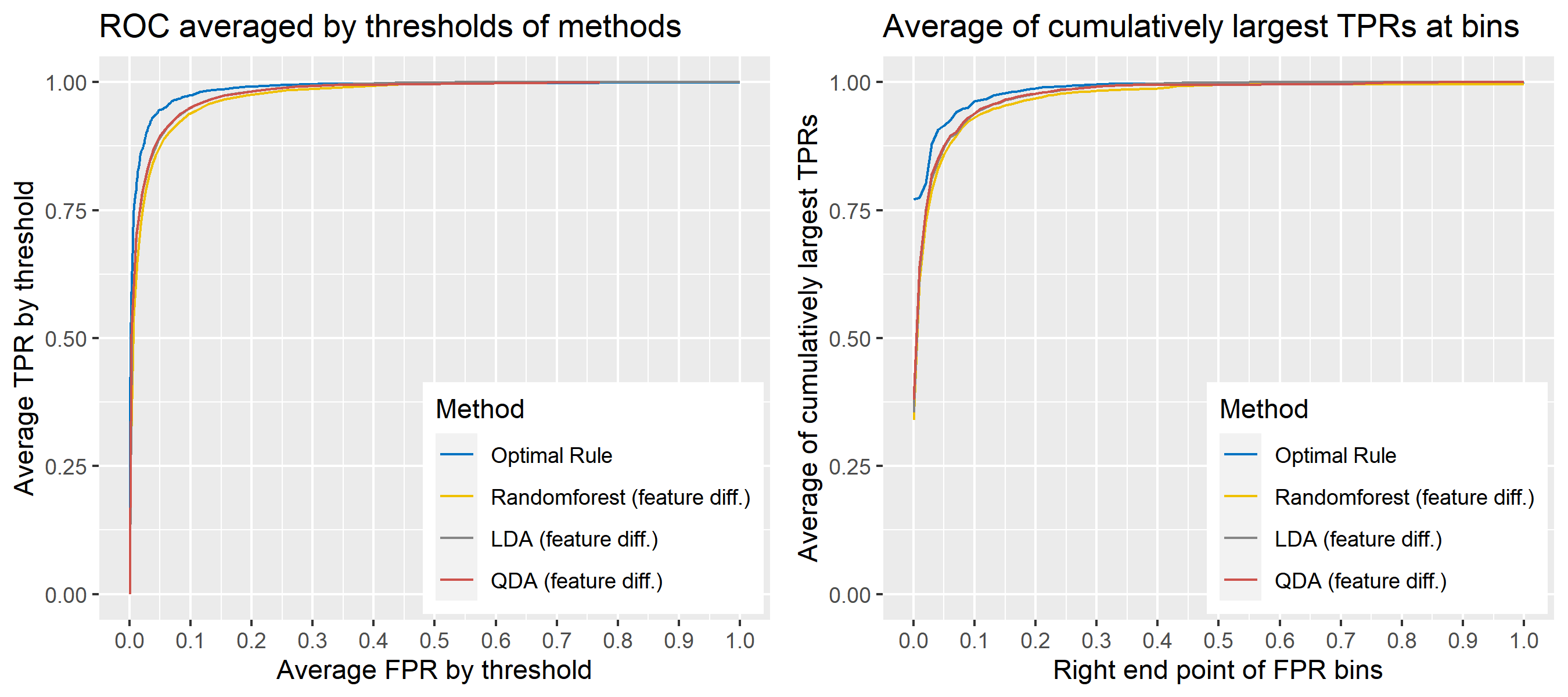
8.5.6.11 Multivariate Result 5
| \[\mbox{Source, }g\] | \[\mu_g\] | \[\Sigma_g\] |
|---|---|---|
| \[1\] | \[\begin{bmatrix} 10&-10&1&8&5 \end{bmatrix}'\] | \[\begin{bmatrix} 16&-4&3&3&3\\-4&25&3&3&3\\3&3&4&2&-0.3\\3&3&2&25&8\\3&3&-0.3&8&9 \end{bmatrix}\] |
| \[2\] | \[\begin{bmatrix} -5&5&-1&12&9 \end{bmatrix}'\] | \[\begin{bmatrix} 9&4&3&3&3\\4&36&3&3&3\\3&3&4&2&-3\\3&3&2&49&2\\3&3&-3&2&9 \end{bmatrix}\] |
| \[3\] | \[\begin{bmatrix} 4&-4&0&20&2 \end{bmatrix}'\] | \[\begin{bmatrix} 16&-9&3&3&3\\-9&25&3&3&3\\3&3&4&1&-0.3\\3&3&1&36&1\\3&3&-0.3&1&9 \end{bmatrix}\] |
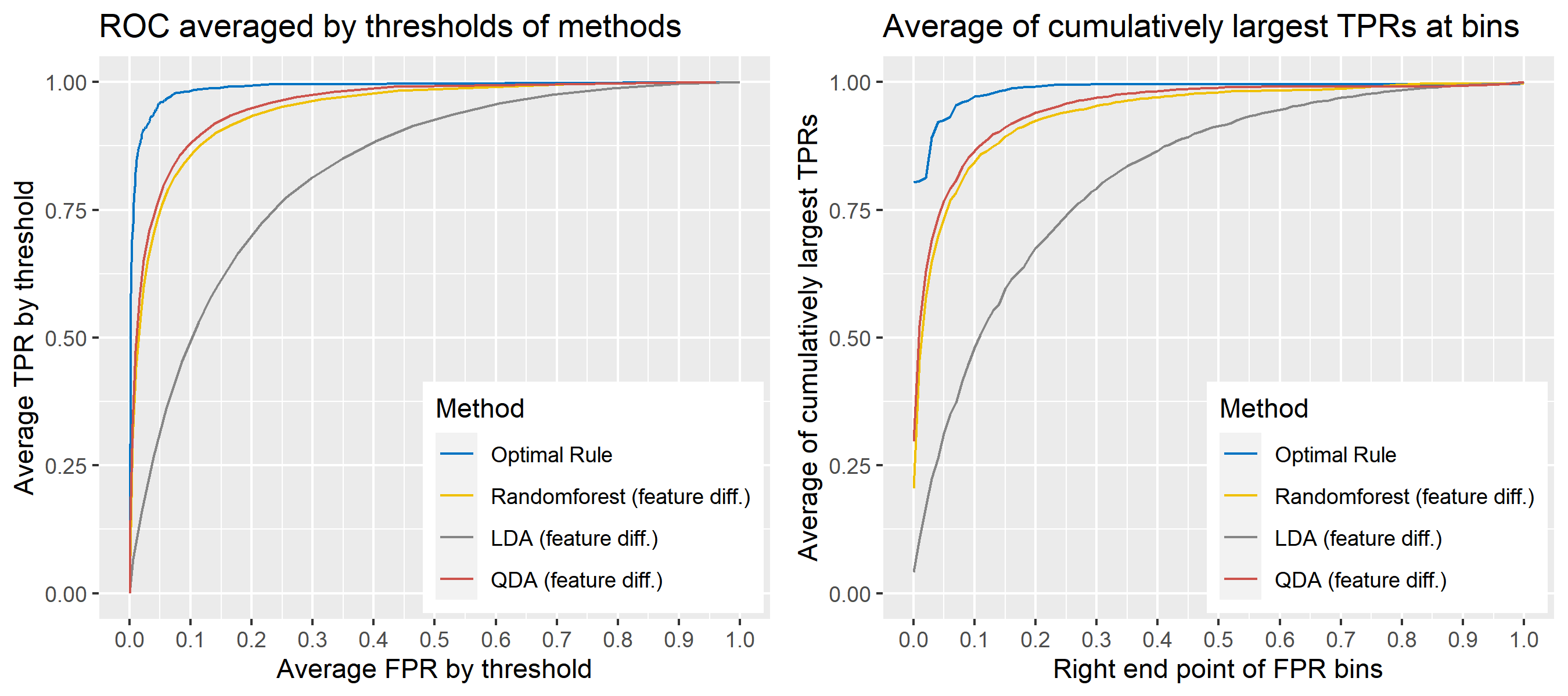
8.5.6.12 Multivariate Result 6
| \[\mbox{Source, }g\] | \[\mu_g\] | \[\Sigma_g\] |
|---|---|---|
| \[1\] | \[\begin{bmatrix} 10&-10 \end{bmatrix}'\] | \[\begin{bmatrix} 25&-4\\-4&25 \end{bmatrix}\] |
| \[2\] | \[\begin{bmatrix} -1&1 \end{bmatrix}'\] | \[''\] |
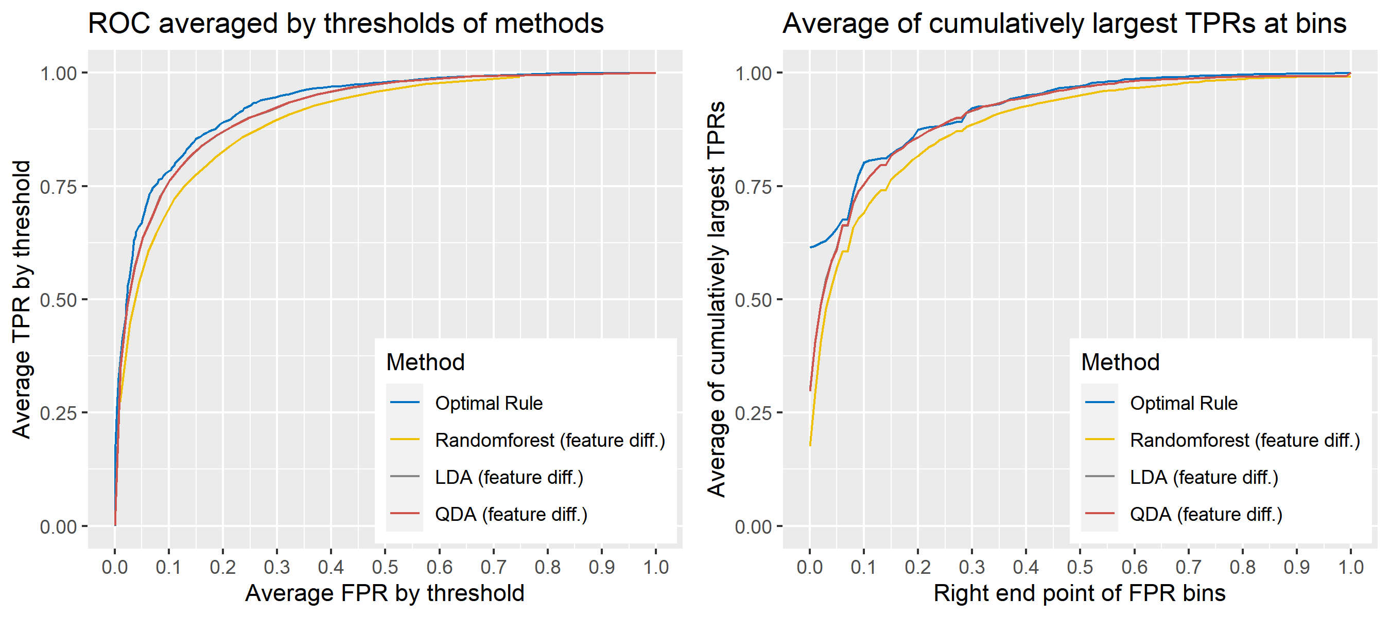
8.5.6.13 Multivariate Result 7
| \[\mbox{Source, }g\] | \[\mu_g\] | \[\Sigma_g\] |
|---|---|---|
| \[1\] | \[\begin{bmatrix} 10&-10 \end{bmatrix}'\] | \[\begin{bmatrix} 25&-9\\-9&36 \end{bmatrix}\] |
| \[2\] | \[\begin{bmatrix} -1&1 \end{bmatrix}'\] | \[''\] |
| \[3\] | \[\begin{bmatrix} 20&-20 \end{bmatrix}'\] | \[''\] |
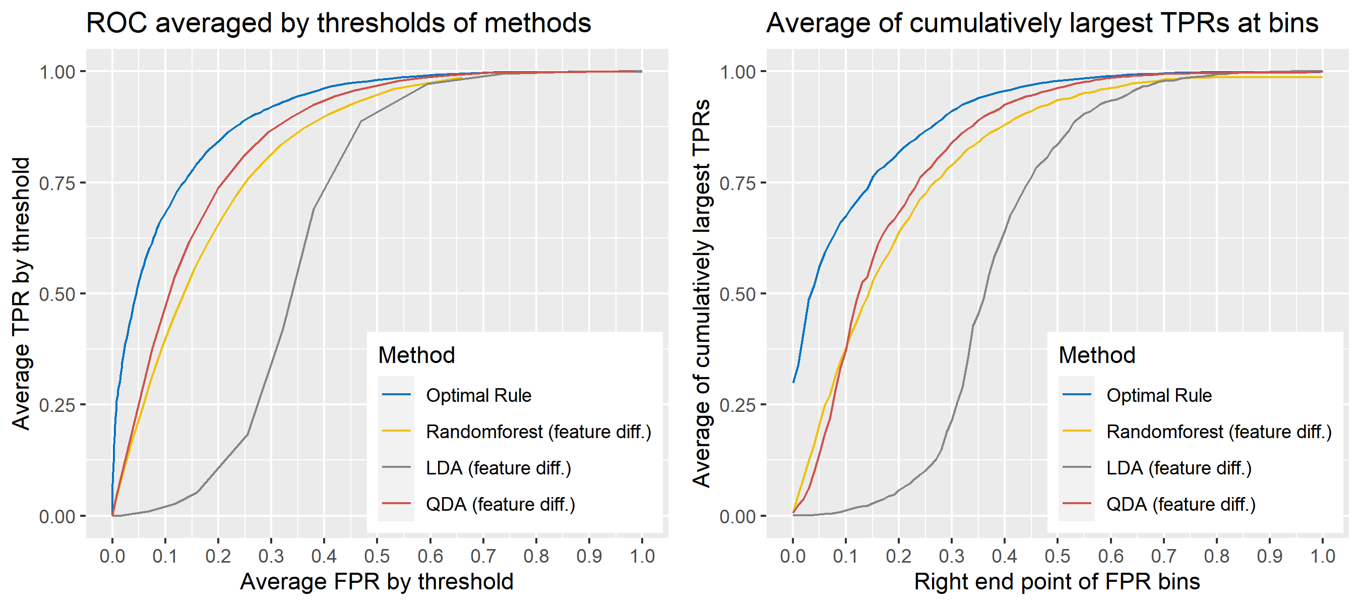
8.5.6.14 Multivariate Result 8
| \[\mbox{Source, }g\] | \[\mu_g\] | \[\Sigma_g\] |
|---|---|---|
| \[1\] | \[\begin{bmatrix} -5&10 \end{bmatrix}'\] | \[\begin{bmatrix} 4&-2\\-2&6 \end{bmatrix}\] |
| \[2\] | \[\begin{bmatrix} -1&6 \end{bmatrix}'\] | \[''\] |
| \[3\] | \[\begin{bmatrix} 0&10 \end{bmatrix}'\] | \[''\] |
| \[4\] | \[\begin{bmatrix} 2&8 \end{bmatrix}'\] | \[''\] |
| \[5\] | \[\begin{bmatrix} -2&7 \end{bmatrix}'\] | \[''\] |
8.5.6.15 Multivariate Result 9
| \[\mbox{Source, }g\] | \[\mu_g\] | \[\Sigma_g\] |
|---|---|---|
| \[1\] | \[\begin{bmatrix} 1&8&5 \end{bmatrix}'\] | \[\begin{bmatrix} 4&0.5&-1\\0.5&9&1\\-1&1&4 \end{bmatrix}\] |
| \[2\] | \[\begin{bmatrix} -1&12&9 \end{bmatrix}'\] | \[''\] |
| \[3\] | \[\begin{bmatrix} 0&20&2 \end{bmatrix}'\] | \[''\] |
8.5.6.16 Multivariate Result 10
| \[\mbox{Source, }g\] | \[\mu_g\] | \[\Sigma_g\] |
|---|---|---|
| \[1\] | \[\begin{bmatrix} 1&10&1&8&5 \end{bmatrix}'\] | \[\begin{bmatrix} 4&-2&-1&-1&-1\\-2&6&-1&-1&-1\\-1&-1&4&0.5&-0.3\\-1&-1&0.5&25&0.5\\-1&-1&-0.3&0.5&9 \end{bmatrix}\] |
| \[2\] | \[\begin{bmatrix} 2&8&-1&12&9 \end{bmatrix}'\] | \[''\] |
| \[3\] | \[\begin{bmatrix} 1&12&0&20&2 \end{bmatrix}'\] | \[''\] |
8.5.7 Real data for simulations
For the simulations in the previous section, data were generated from normal distributions, and optimal rule outperformed the other methods under the condition. To examine if it works well in practice, we compare it with the other techniques on the glass data published in this paper where the data are referred to as Dataset 3.
8.5.7.1 Data description
We use the data set consisting of 31 and 17 glass panes (AA, AB, …, AAQ, AAR / BA, BB, …, BP, BR) provided from company A and B, and 22 to 24 fragments were randomly sampled frome each source, a glass pane. A single fragment as an observational unit has the average amount of concentration for 18 chemical elements such as Li7, Na23, and Mg25 where the mean was caluated from repeatedly measured values of concentration. Hence, each row of the data at our analysis level is made up of a 18-dimensional vector whose coordinates indicate the average amount of concentration for the 18 chemical elements, and extra information like which source fragments came from.
8.5.7.2 Simulation plan for glass data
The basic scheme is the same as the explanation in Simulation plan, the section above, but there are some differences. For the glass data, 20 random splits of a dataset will be generated into test sets so that an average ROC curve aggregated from 20 ROC curves can be provided. Specifically, 6 observations per source are assigned to a test set, and the rest is assigned to a training set. Then, 16 to 18 fragments per a source remain in a training set, which is not enough to estimate 18 by 18 covariance matrix for each source, and covariance estimation is a necessary process for optimal rule. Alternatively, we use pooled covariance estimate for optimal rule with the glass data. One way is to use a single pooled covariance across all sources, and another one is apply separate pooled covariance estimate for each company. The latter is based on our prior belief that covariance structure could differ by company, and could be similar within the same company while there is the possibility that a single sample covariance across all sources is more reliable than separate ones.
Besides, unlike the other methods, randomforest method needs to train its model while the other methods just computes their matching rule based on summary statistics. Since feature differences are calculated from all pairwise observations in a training set, a serious imbalance to the number of pairs from the same sources, and that from different sources happens as the number of sources and the number of observations increase. To address some potential problems due to the imbalance, we also employ downsampling technique to randomforest method where twice the number of pairs from the same sources is randomly selected from different sources instead of utilizing all pairs from different sources.
Lastly, subsets of the whole data will be used to compare mathing techniques where a subset of data is determined by choosing different glass panes. For example, we can apply matching methods to a dataset with 6 different panes (AA, AB, AC, BA, BB, and BC) as the whole data. In this report, a scenario will be based on a subset of the entire glass data, and several scenarios will be presented.
To sum up, two kinds of average of 20 ROC curves will be presented for each scenario: average of the values of TPRs and FPRs by threshold value, and average of cumulatively largest vause of TPR in each bin for FPR. Optimal rule’s performance will be compared with LDA, QDA, and randomforest based on feature differences as before, but optimal rule and randomforest have two different scenarios. For optimal rule, one is to apply a single pooled covariance across all sources, and the other is to use separate pooled covariance for each company. Randomforest will present a regualr one without downsampling, and one with downsampling. Consequently, there will be 6 methods compared.
8.5.8 Simulation results using glass data
8.5.9 Extension to openset problems
This is motivated to consider the situations where no training data are given for questioned evidence such as glass fragments. In earlier work, we assumed finite known sources corresponding to a closed-set situation. The assumption would break as a questioned evidence does not belong to those known sources. To improve this weakness, and move to openset framework, we used simple hierarchical structure first.
8.5.9.1 Initial set-up
\[X|\mu, Y|\mu \sim N(\mu, \Sigma) \mbox{ where }\mu \sim N(M, V), \ X, Y \mbox{ are conditionally independent}\]
\[\begin{align*} &P(\mbox{the same source error}) \\ &= \iint_{T_{SS}}\iint_{\mathbb{R}^2} f_X(x|\mu_X)f_Y(y|\mu_Y)h(\mu_X)h(\mu_Y) d\mu_X d\mu_Y dx dy \\ &= \iint_{T_{SS}}\iint_{\mathbb{R}^2} (2\pi)^{-1}\Sigma^{-1}\exp{\left(-\frac{(x - \mu_X)^2}{2\Sigma}\right)}\exp{\left(-\frac{(y - \mu_Y)^2}{2\Sigma}\right)}\times \\ &(2\pi)^{-1}V^{-1}\exp{\left(-\frac{(\mu_X - M)^2}{2V}\right)}\exp{\left(-\frac{(\mu_Y - M)^2}{2V}\right)}d\mu_X d\mu_Y dx dy\\ &= \iint_{T_{SS}} \mbox{MVN}\left(\left(\begin{matrix}M \\ M\end{matrix}\right), \left(\begin{matrix}\Sigma + V & 0 \\ 0 & \Sigma + V \end{matrix} \right) \right) dxdy \end{align*}\]
\[\begin{align*} &P(\mbox{different source error}) \\ &=\iint_{T_{DS}}\iint_{\mathbb{R}^2} f_X(x|\mu)f_Y(y|\mu)h(\mu)d\mu d\mu_Y dx dy \\ &=\iint_{T_{DS}}\iint_{\mathbb{R}^2} (2\pi)^{-1}\Sigma^{-1}\exp{\left(-\frac{(x - \mu)^2}{2\Sigma}\right)}\exp{\left(-\frac{(y - \mu)^2}{2\Sigma}\right)} \times\\ &(2\pi)^{-1/2}V^{-1/2}\exp{\left(-\frac{(\mu - M)^2}{2V}\right)}d\mu_X d\mu_Y dx dy \\ &=\iint_{T_{DS}} \mbox{MVN}\left(\left(\begin{matrix}M \\M\end{matrix}\right), \left(\begin{matrix}\Sigma + V & V \\ V & \Sigma + V \end{matrix} \right) \right) dxdy \end{align*}\]
\[\begin{align*} &P(\mbox{the same source error})(1-w) + P(\mbox{different source error})w\\ &=\iint_{T_{SS}} \mbox{MVN}\left(\left(\begin{matrix}M \\M\end{matrix}\right), \left(\begin{matrix}\Sigma + V & 0 \\ 0 & \Sigma + V \end{matrix} \right) \right) dxdy (1-w)\\ &+ \iint_{T_{DS}} \mbox{MVN}\left(\left(\begin{matrix}M \\M\end{matrix}\right), \left(\begin{matrix}\Sigma + V & V \\ V & \Sigma + V \end{matrix} \right) \right) dxdy w \\ &= \iint_{T_{SS}} \mbox{MVN}\left(\left(\begin{matrix}M \\M\end{matrix}\right), \left(\begin{matrix}\Sigma + V & 0 \\ 0 & \Sigma + V \end{matrix} \right) \right) dxdy (1-w) + \\ &w - \iint_{T_{SS}} \mbox{MVN}\left(\left(\begin{matrix}M \\M\end{matrix}\right), \left(\begin{matrix}\Sigma + V & V \\ V & \Sigma + V \end{matrix} \right) \right) dxdy w \\ &= w + \iint_{T_{SS}} \mbox{MVN}\left(\left(\begin{matrix}M \\M\end{matrix}\right), G_1 \right)(1-w) - \mbox{MVN}\left(\left(\begin{matrix}M \\M\end{matrix}\right), G_2 \right) w dxdy\\ &\mbox{where } G_1 = \left(\begin{matrix}\Sigma + V & 0 \\ 0 & \Sigma + V \end{matrix} \right), G_2 = \left(\begin{matrix}\Sigma + V & V \\ V & \Sigma + V \end{matrix} \right) \end{align*}\]
\[\begin{align*} T_{SS}^{Opt} = \left\{(x,y):\ \exp{\left(-\frac{1}{2} \left(\begin{matrix}x - M \\y - M \end{matrix}\right)'\left(G_1^{-1} - G_2^{-1}\right)\right)}\left(\begin{matrix}x - M \\y - M \end{matrix}\right) < \frac{w}{1-w} \left|G_1\right|^{1/2}\left|G_2\right|^{-1/2}\right\} \end{align*}\] , which is valid for both univariate and multivariate cases.
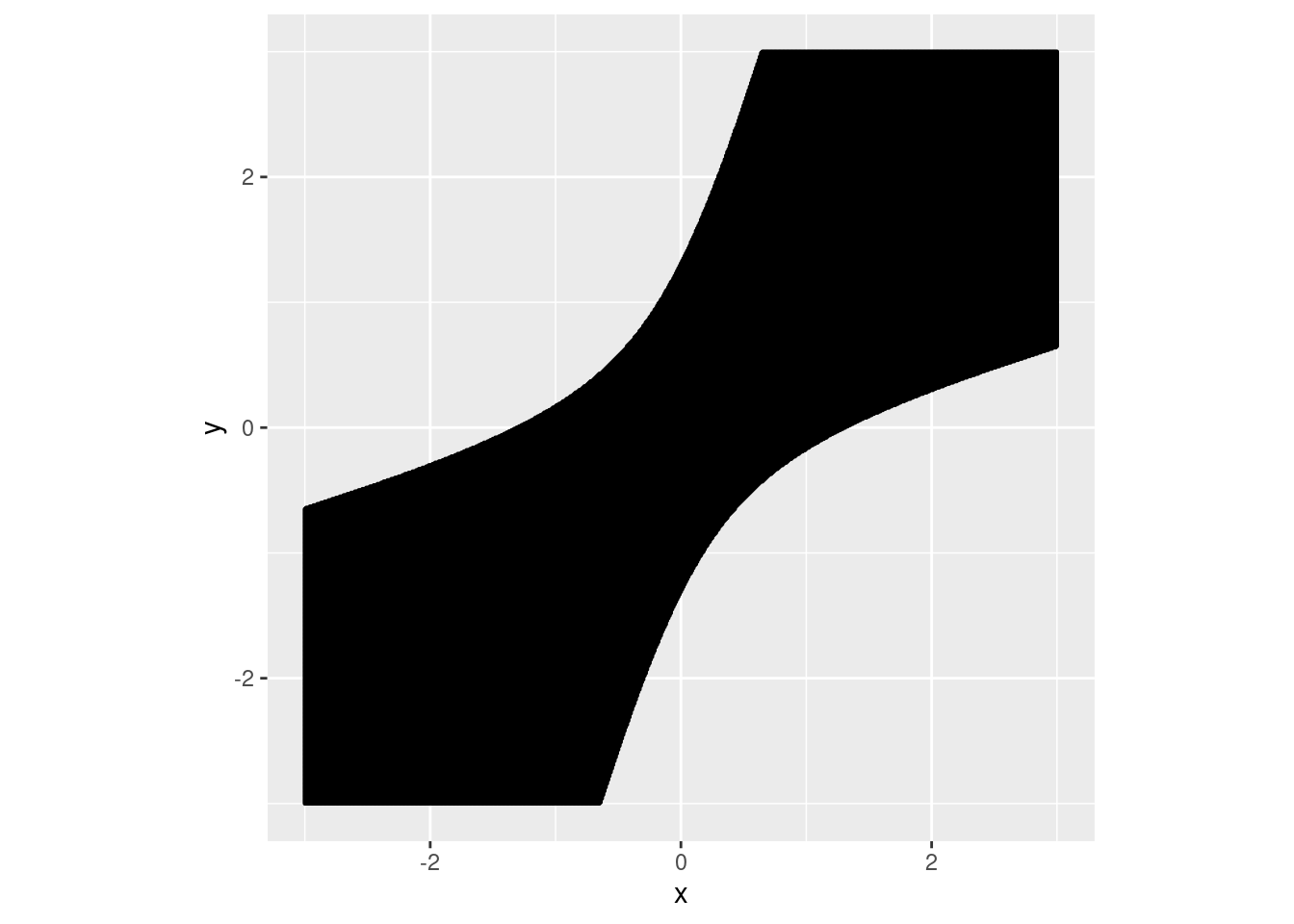
8.5.9.2 An example based on normal populations
Set-up: \(X|\mu, Y|\mu \sim \mbox{N}(\mu, \Sigma = 1)\) where \(\mu \sim \mbox{N}(M = 0, V =1)\), which results in \(X, Y \sim N(0,2)\).
8.5.9.3 Application to glassdata
Assumption: \[X|\mu, Y|\mu \sim N(\mu, \Sigma) \mbox{ where }\mu \sim N(M, V), \ X, Y \mbox{ are conditionally independent.}\]
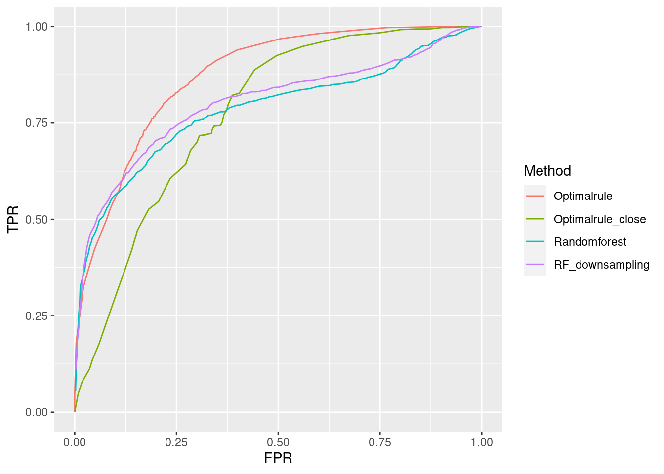
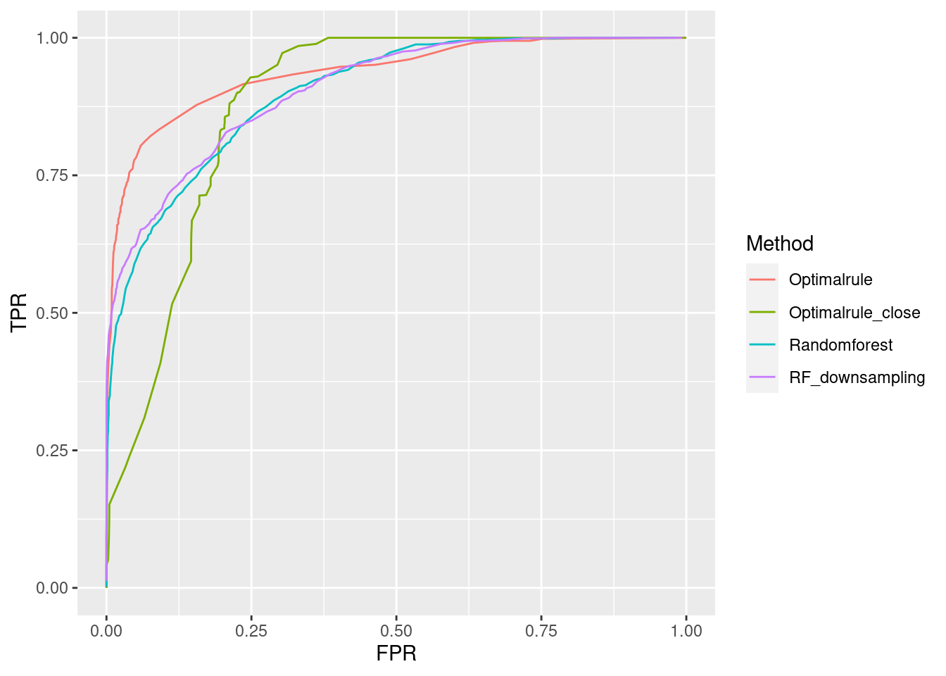
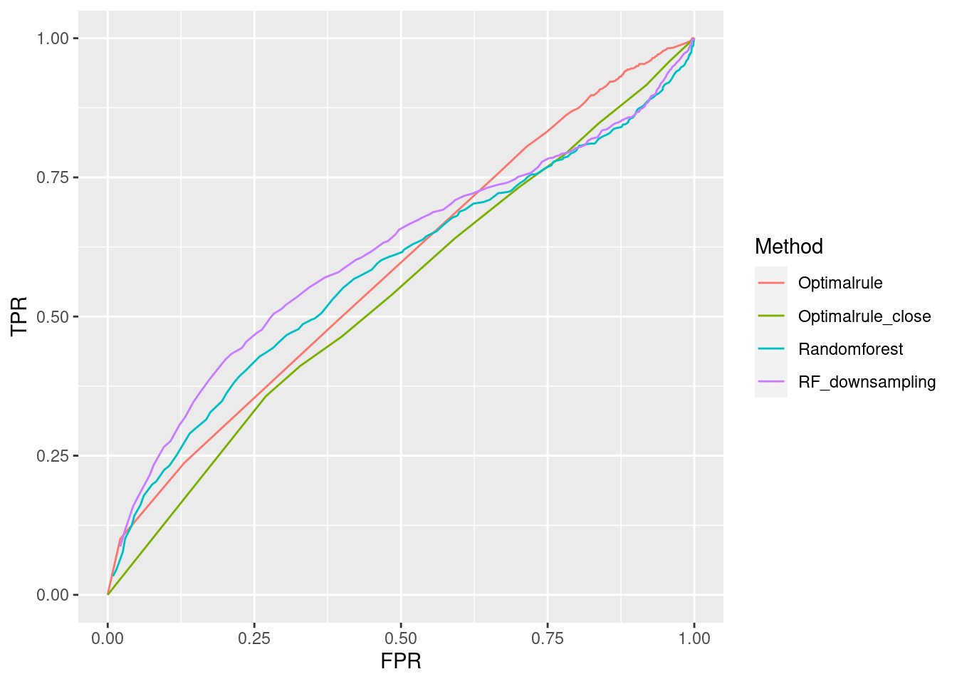
Here, \(\Sigma\) is replaced with a pooled sample covariance based on training data. For \(M\) and \(V\), we use the overall sample mean, and the sample covariance of sample means by source based on training data as well. Actually, the sample means and covariance matrices are so different by company that produced glass panes. The names of panes started with letters A, B indicates their production from the company A and B, respectively.
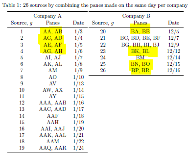
- Training: AA(1/3), AC(1/4), AE(1/5), AG(1/6)
- Testset: AB(1/3), AD(1/4), AF(1/5), AH(1/6)
- Training: BA(12/5), BK(12/12), BN(12/15), BP(12/16)
- Testset: BB(12/5), BL(12/12), BO(12/15), BR(12/16)
- Training: AA(1/3), AC(1/4), AE(1/5), AG(1/6)
- Testset: AI(1/7), AJ(1/7), AK(1/8), AL(1/8)
- Training: AA(1/3), AC(1/4), AE(1/5), AG(1/6), BA(12/5), BK(12/12), BN(12/15), BP(12/16)
- Testset: AB(1/3), AD(1/4), AF(1/5), AH(1/6), BB(12/5), BL(12/12), BO(12/15), BR(12/16)
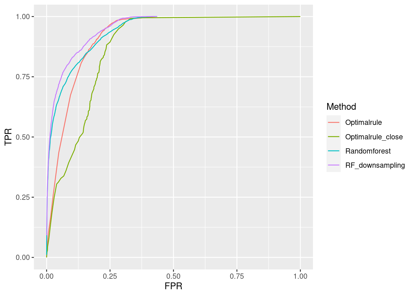
- Training: AA(1/3), AC(1/4), AE(1/5), AG(1/6))
- Testset: BA(12/5), BK(12/12), BN(12/15), BP(12/16)
- Training: AI(1/7), AJ(1/7), AK(1/8), AL(1/8)
- Testset: AV(1/13), AY(1/15), AAA(1/16), AAC(1/17)
8.6 SRL behavior and dependence
The following projects dealt with examining SLR behavior and performance. Project 1 examines the use of SLR for forensic glass. Besides performance metrics, the paper addresses the issue of the dependence on the training data selected.
Project 2 examines the dependence structure generated when pairwise comparisons are used.
8.7 Project 1. Evaluation of SLR for glass data
In forensic settings, likelihood ratios (LR) are used to provide a numerical assessment of the evidential strength but require knowing a complex probability model, particularly for pattern and impression evidence. A proposed alternative relies on using similarity scores to develop score-based likelihood ratios (SLR). We illustrate the use of simulations to evaluate feature-based LR and SLR already present in the literature focusing on a less-discussed aspect, dependence on the data used to estimate the ratios.We provide evidence that no clear winner outperforms all other methods through our simulation studies. On average, distance-based methods of computing scores resulted in less discriminating power and a higher rate of misleading evidence for known non-matching data. Machine learning-based scores produce highly discriminating evidential values but require additional samples to train. Our results also show that non-parametric estimation of score distributions can lead to non-monotonic behavior of the SLR and even counter-intuitive results. We also present evidence that the methods studied are susceptible to performance issues when the split into training, estimation and test sets is modified. The resulting SLRs could even lead examiners in different directions.
8.7.1 Communication of Results
You can find the results of this project formatted as a creative component here
Previous stages were presented in poster sessions:
- “An evaluation of score-based likelihood ratios for glass data.”
February 2021
Authors: Federico Veneri and Danica Ommen
American Academy of Forensic Sciences, Virtual
Click for Poster Image

Previous stages were presented in poster sessions:
- “An evaluation of score-based likelihood ratios for glass data.”
May 2022
Authors: Federico Veneri and Danica Ommen
CSAFE All Hands
Click for Poster Image
8.8 Project 2. Ensemble of SLR systems for forensic evidence.
Previous stages were presented in poster sessions and talks:
- “Machine Learning Methods for Dependent Data Resulting from Forensic Evidence Comparisons”
August 2021
Authors: Danica Ommen and Federico Veneri.
Joint Statistical Meeting
- “Ensemble of SLR systems for forensic evidence.”
February 2022
Authors: Federico Veneri and Danica Ommen
American Academy of Forensic Sciences, Virtual
Click for Poster Image

- “Ensemble of SLR systems for forensic evidence.”
May 2022
Authors: Federico Veneri and Danica Ommen
CSAFE All Hands
Click for Poster Image

- “Ensemble of SLR systems for forensic evidence.”
August 2022
Authors: Federico Veneri and Danica Ommen
Joint Statistical Meeting
Next!
8.8.0.1 Abstract:
Machine learning-based Score Likelihood Ratios have been proposed as an alternative to traditional Likelihood Ratio and Bayes Factor to quantify the value of forensic evidence. Scores allow formulating comparisons using a lower-dimensional metric [1]., which becomes relevant for complex evidence where developing a statistical model becomes challenging
Although SLR has been shown to provide an alternative way to present a numeric assessment of evidential strength, there are still concerns regarding their use in a forensic setting [2]. Previous work addresses how introducing perturbation to the data can lead the forensic examiner to different conclusions [3].
Under the SLR framework, a (dis)similarity score and its distribution under alternative propositions is estimated using pairwise comparison from a sample of the background population. These procedures often rely on the independence assumption, which is not met when the database consists of pairwise comparisons.
To remedy this lack of independence, we introduce an ensembling approach that constructs training and estimation sets by sampling forensic sources, ensuring they are selected only once per set. Using these newly created datasets, we construct multiple base SLR systems and aggregate their information into a final score to quantify the value of evidence.
8.8.1 Introduction to the forensic problem.
Score likelihood ratios (SLR) are an alternative way to provide a numerical assessment of evidential strength when contrasting two propositions. The SLR approach focuses on a lower-dimensional (dis)similarity metric and avoids distributional assumptions regarding the features (Cite)
Consider the hypothetical case of a common source problem in forensics that could come up in different forensic domains.
| Forensic glass problem | Forensic handwriting problem |
|---|---|
| A glass was broken during a break in | A stalking victim received two handwriting notes within a week |
| Two individuals (PoI) arrested, and one glass fragment recovered from each. | Trying to determine if there are two potential stalker the forensic expert may be asked: |
| Q: Do these two glass fragments come from the same window? | Q: Are we dealing with the same writer? |
In both scenarios, we can state two propositions we can try to evaluate.
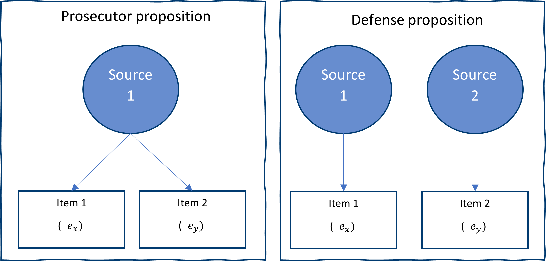
Hp) The source associated with item 1 is the same as the source related to item 2.
Hd) The sources from each item are different.
In the forensic problems describe we would have the following data \(E=\{e_{x}, e_{y},e_A\}\) where:
\(e_x\) the first item
\(e_y\) the second item
\(e_A\) background population sample.
For each element some features are measured and recorder. Let’s denote \(u_x\), \(u_y\) as the vector of measurements for \(e_x\) and \(e_y\) . And let \(A_{ij}\) be the measurement taken in the background population where \(i\) indexes a sources and \(j\) indexes items within source.
Under the prosecutor proposition, \(e_x\) and \(e_y\) have been generated from the same source while under the defense proposition they have been sampled from two independent sources.
8.8.1.0.1
Propositions
8.8.1.0.3 Common source in handwriting
In the case of handwriting problem the data consist of two questioned documents (QD) \(e_𝑥\), \(e_𝑦\). We can re write the proposition as:
\(𝐻_𝑝\): \(e_𝑥\) and \(e_𝑦\) were written by the same unknown writer.
\(𝐻_d\): \(e_𝑥\) and \(e_𝑦\) were written by two different unknown writers.
Traditional approach for questioned document comparison is based on visual inspection by trained expert who identify distinctive traits. CSAFE approach [5,6] decompose writing samples into graphs, roughly matching letter and assign each them into one of 40 cluster. Cluster frequency has been used as a feature to answer the common source problem [6] since documents written by the same writer are expected to share similar cluster profiles.
Let \(𝑢_𝑥\) and \(𝑢_𝑦\) be the cluster frequencies from \(e_𝑥\) and \(e_𝑦\) respectively. In this problem background measurement are taken from documents generated by known writers to construct the SLR system
\[ A=\{A_{ij}:𝑖^{𝑡ℎ} 𝑤𝑟𝑖𝑡𝑒𝑟, 𝑗^{𝑡ℎ} 𝑑𝑜𝑐𝑢𝑚𝑒𝑛𝑡\} \]
Pairwise comparisons are created from the set 𝑨 and classified as known match (KM) or known non match (KNM).
8.8.2 The dependence problem in SLR.
The forensic proposition can be translated into sampling models that generated the data \(𝑀_𝑝\) and \(𝑀_𝑑\) respectively to define training and estimation set [3].
In the case of data \(𝑀_𝑝\) comparisons from the same known source or KM (\(𝑪_{𝑪𝑺_𝑷}\)) are used, while in the case of \(𝑀_𝑑\) comparisons from different sources (\(𝑪_{𝑪𝑺_D}\)) or KNM are used.
| Under \(𝑀_𝑝\), KM are used: | Under \(𝑀_𝑑\), KNM are used: |
|---|---|
| \(𝑪_{𝑪𝑺_𝑷}= \{𝑪(𝑨_𝒊𝒋,𝑨_𝒌𝒍): 𝒊=𝒌\}\) | \(𝐶_{𝐂𝐒_𝑫}=\{𝐶(𝐴_𝑖𝑗,𝐴_𝑘𝑙): 𝑖≠𝑘\}\) |
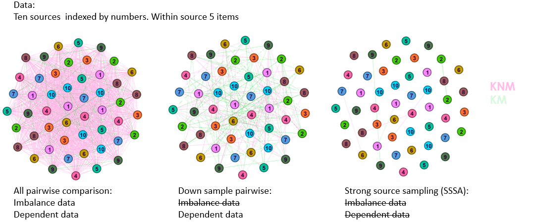
At a source level, sources are compared multiple times. In \(𝑪_{𝒄𝒔_𝑷}\) : multiple within comparisons uses the same source, In \(𝐶_{𝑐𝑠_𝐷}\) : multiple between comparison use the same sources and lastly same source appears in both comparisons sets.
At an item level, same items are compared multiple times. e.g., \(𝑪(𝑨_{𝟏𝟏},𝑨_{𝟐𝟏} ),𝑪(𝑨_{𝟏𝟏},𝑨_{𝟑𝟏} )\)
The issue is that machine learning-based comparison metrics and density estimation procedures rely on the independence assumption, but this assumption is not met.
Practitioner often uses \((𝑪_{𝒄𝒔_𝑷},𝑪_{𝒄𝒔_D})\) directly while developing an SLR system. To illustrate how convoluted this comparison can be we present the following figure to illustrate the dependence structure of pairwise comparison and some solutions.
8.8.3 Methology.
8.8.3.1 Traditional SLR.
We define as traditional SLR the construction of a SLR system using a down sampling approach. First, the background data is split into training and estimation, within each set all pairwise comparisons are constructed and features are created.
We consider as features…
Since the number of known non matches outnumber known matches a down sample step is used have a balanced data set. For comparison metric we trained a Random forest (cite)
However, this approach has several drawbacks. ML method and density estimation procedures assume that we have iid. That is not the case, since when comparisons are made, items enter comparison multiple times. In addition, in theory the sample used for estimating the SLR should consist of independently sampled sources for both KM and KNM. When we construct all the pairwise comparison, sources are compared multiple times, hence we are violating the independence assumption.
To resolve this issue, we propose sampling sources restricting the possibility of a source beings used multiple times. This greatly reduced the sample size available but results in a situation closer to our theoretical results, in addition, during a second stage we propose using aggregations inspired in ensemble learning to improve the performance of the SLR.
8.8.3.2 Ensemble SLR.
As in ensemble learning the idea behind constructing base score likelihood ratio (BSLR) is training the model with a partition of the data and then combining them into a final score.
8.8.3.2.1 Sampling Algorithms
To generate independent set we introduce sampling algorithms that can construct set were assumptions are met.We denote the first version as the Strong Source Sampling Algorithm (SSSA) to generate independent training and testing data.
| Strong Source Sampling Algorithm (SSSA) |
|---|
|
| Result: A pairwise database where sources and items are not compared multiple times |
A less strict algorithm we denote as Weak Source Sampling Algorithm (WSSA) were comparison are sampled such that items are compared only once.
| Weak Source Sampling Algorithm (SSSA) |
|---|
|
| Result: A pairwise database where items are not compared multiple times |
On our current implementation we use a Fast version of the sampling algorithms which in essence reproduce the results but avoids looping over the data.
8.8.3.2.2 Base SLR (BSLR).
The sampling algorithms can be used to construct set for constructing comparison metrics and their distribution as follows:
| Base Score Likelihood Ratio (BSLR) |
|---|
For 1:M
|
| Result: M- Base Score Likelihood Ratios (BSLR) |
8.8.3.2.3 Ensemling BSLRs (ESLR)
The previous process generated M-BSLRs that need to be combined into a final prediction. Let \(SLR_{im}\) denote the case of the i-th observation in the validation set and the log10 output value for the m-th BSLR.
We can organize our predictions into a matrix were each row represents an observation and there are \(M\) columns each associated with a particular BSLR.
We consider Naïve ways of combining the information.
The mean ESLR: consist of taking the mean across predictions for the same ith observation
The median ESLR: consist of taking the median
Vote ESLR: consist of translating the prediction to categories and use majority voting.
If an additional set is available, additional step can be done.
We consider an optimization step, where our M-BSLRs are evaluated according to some performance metric. As metrics we considered
Cost function (\(CLLR\))
Rate of misleading evidence for KM (\(RME_{KM}\) )
Rate of misleading evidence for KMN (\(RME_{KNM}\))
Discriminatory power for KM (\(DP_{KM}\))
Discriminatory power for KMN (\(DP_{KNM}\))
Note that the best SLR would minimize the CLLR, and both RME while maximizing the DP. We can compute weights that assign more importance to BSLRs that have a better performance for each metric.
The previous approach is univariate, i.e. optimize one dimension. So we consider a combined weight for \(RME\) and \(DP\).
Lastly we consider a logistic calibration approach or fusion.
- Fusion: Over the optimization set, a GLM is trained to combine the M-BSLR into a final score.
8.8.4
8.8.5 Experimental set up
8.8.5.1 Data
We use CSAFE and VCL handwriting data to show case our approach. From the raw data, clustering templates are used to classify each graph into one of the 40 clusters then, the proportion of graphs in each cluster is computed for each writer and prompt. This process generates the relative cluster data.
In the case of traditional SLR, we used the London letter prompt for training and estimation. While in the case of the Ensemble SLR, when they require and aditional optimization set a down sample version of the Wizard of Oz prompt was used.
As validation set, we consider the VCL prompt. This database was collected in a different study and it is highly unlikely that CSAFE and VCL database contains the same writers.
[Summary Stats 1]
8.8.5.2 Experiment 1
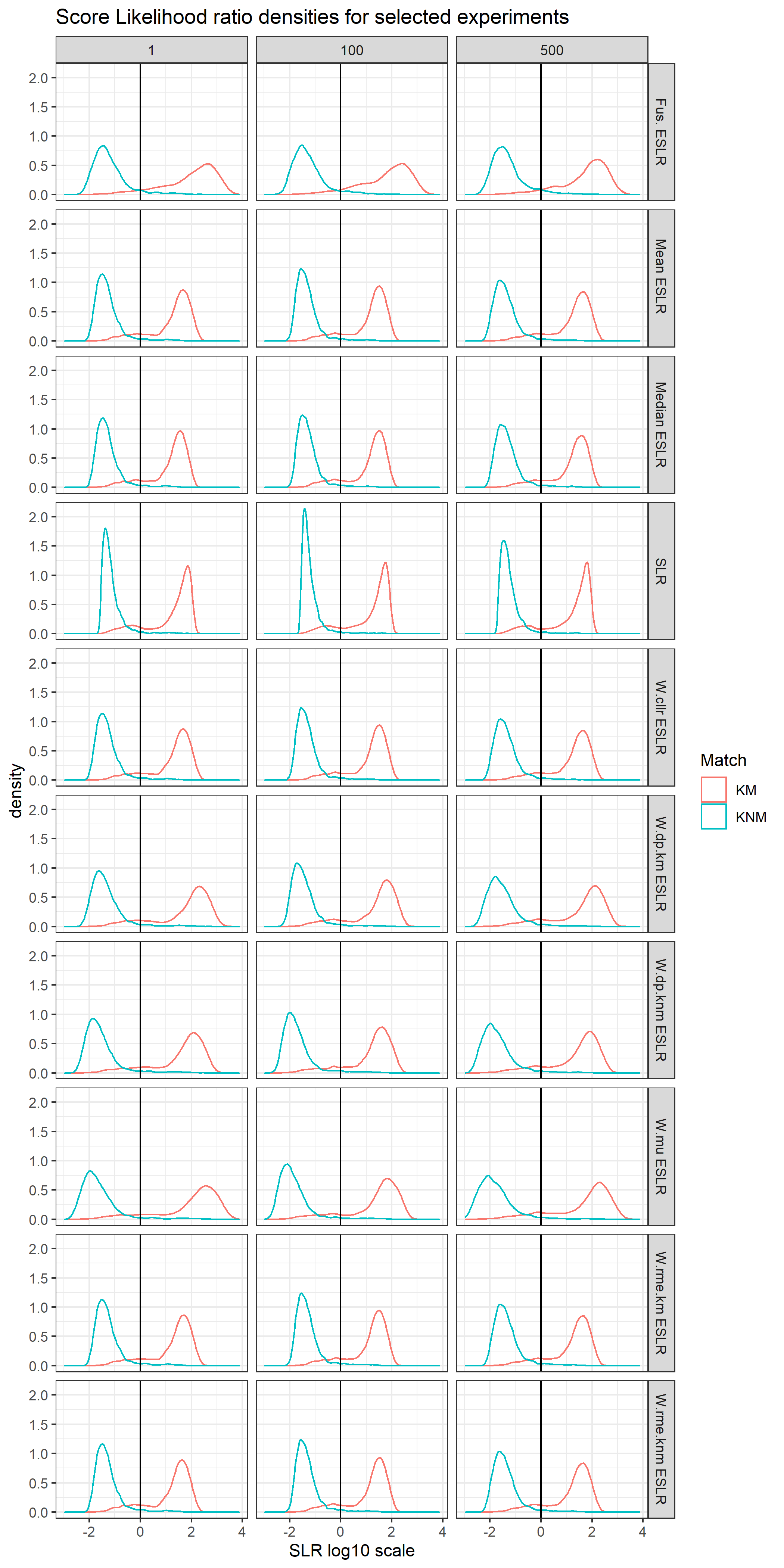
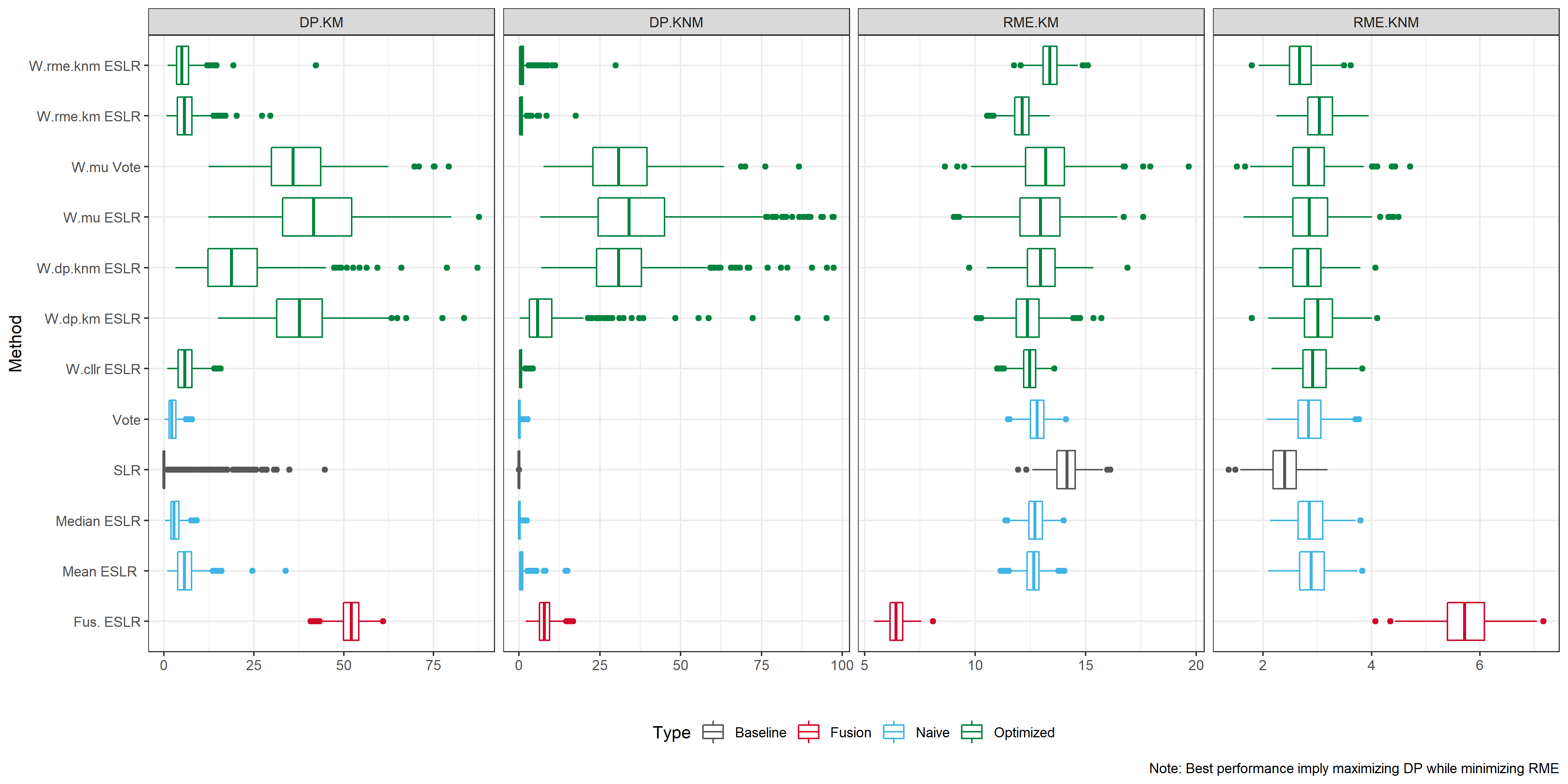
To illustrate our approach, we simulate 500 repetition of the following experiment.
In each experiment 100 BSLR are trained using SSSA over CSAFE London prompts.
Optimization set are generated down sampling from CSAFE Wizard of Oz prompts
Validation set are generated downs sampling VCL prompts.
Our Final values consist of:
Baseline SLR
Naïve ESLR : Voting, mean and median
Optimized ESLR over: Cllr, RME KM/KNM, DP KM/KNM, Multi criteria and fusion.
For this SLR performance metrics are computed in each experiment.
8.8.6 What we would like to evalaute? (and how we measure it).
Adapted from CC
Does the outcome lead the juror in the correct direction?
SLRs provide a numerical value that experts can interpret as evidence supporting the prosecutor or defense proposition.
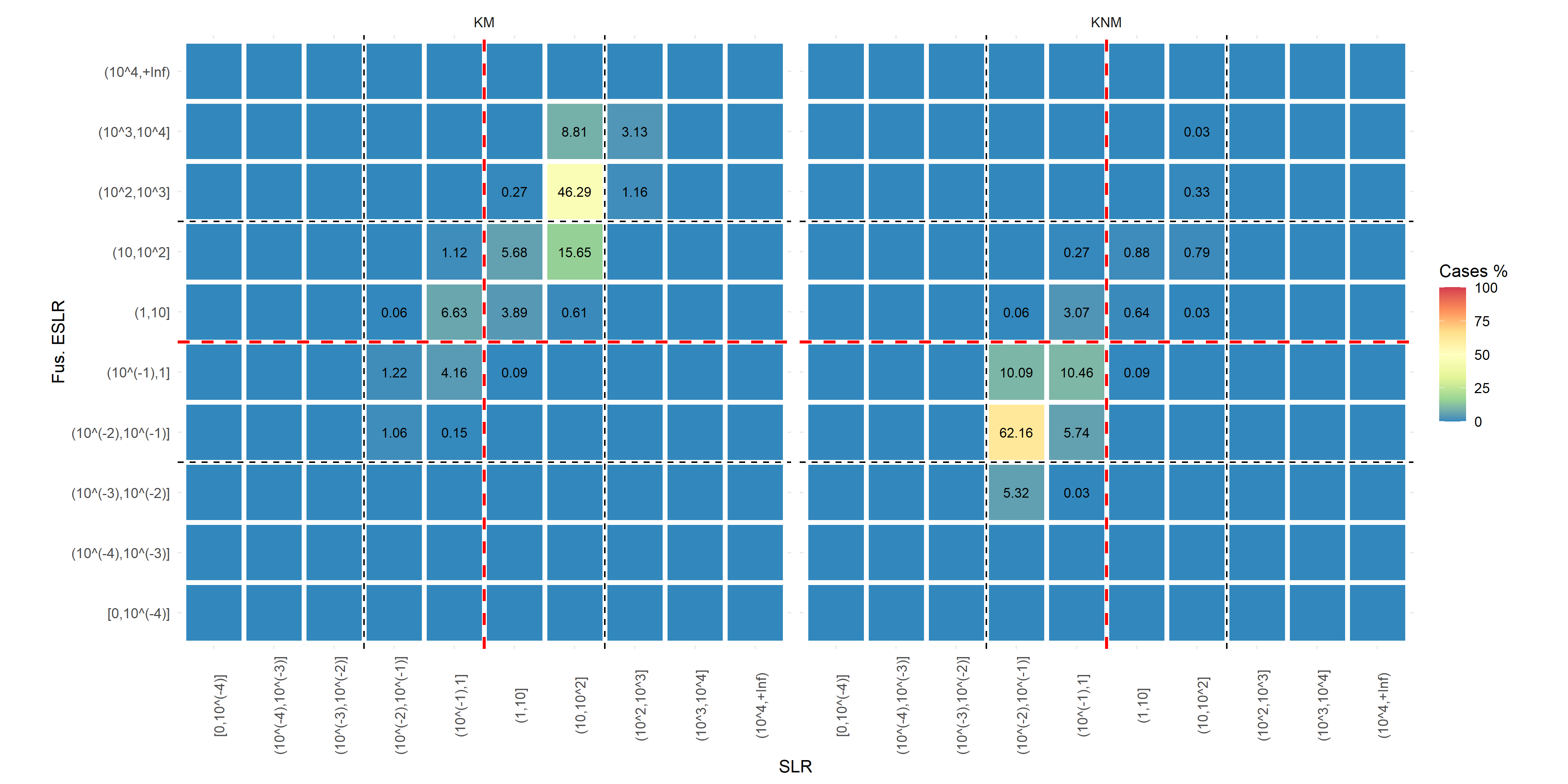
KNM KM SLR <1 (Evidence towards Hd) Correct Misleading SLR >1 (Evidence towards Hp) Misleading Correct We consider misleading evidence results that would lead the juror in the incorrect direction and compute:
RME for KM: The percentage of KM that present a SLR<1
- \(\sim\) False non matches/ false negatives
RME for KNM: The percentage of KNM that present a SLR>1
- \(\sim\) False matches / false positives
A good SLR system would present low values of RME.
Are the methods capable of providing strong evidence in the correct direction?
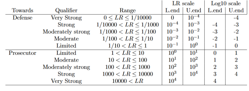
We can translate numeric values into the vebral scale recommend to present forensic findings. We would like our SLR system to be able to discriminate between propositions with ‘enough’ strength
We consider:
DP for KM: The percentage of KM that present a SLR>100
DP for KNM: The percentage of KNM that present a SLR<1/100
A good SLR system would present high values of discriminatory power.
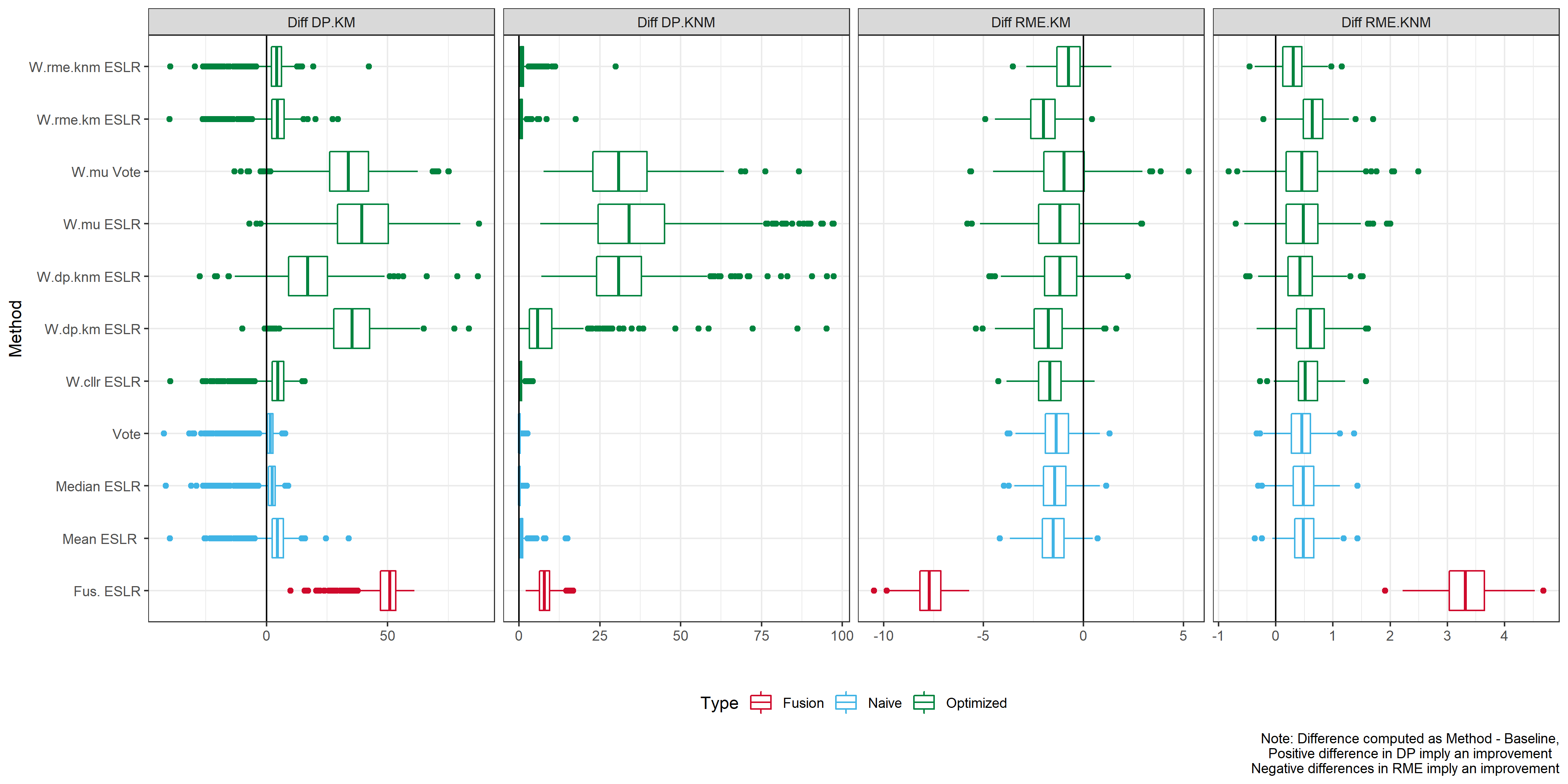
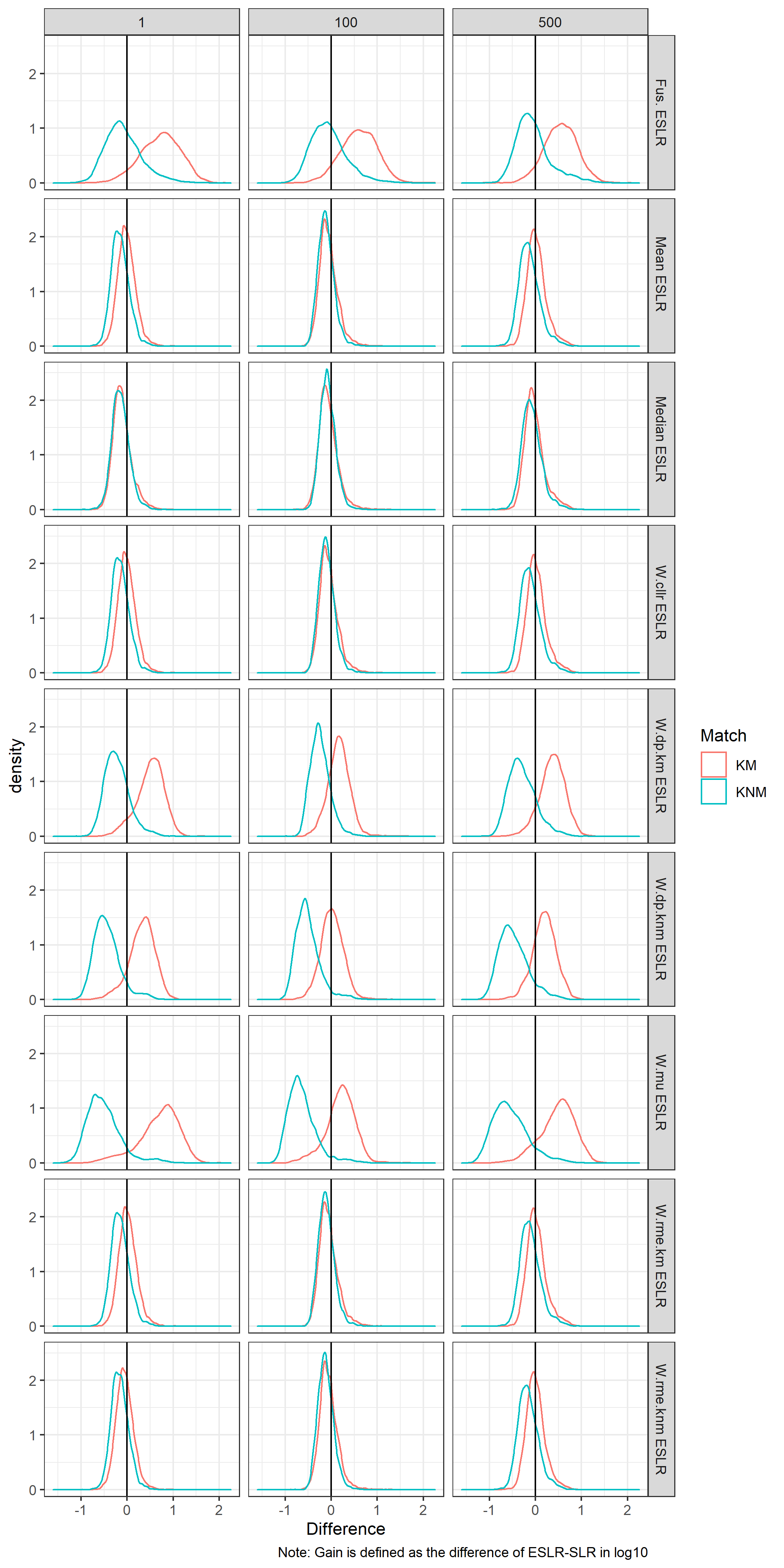
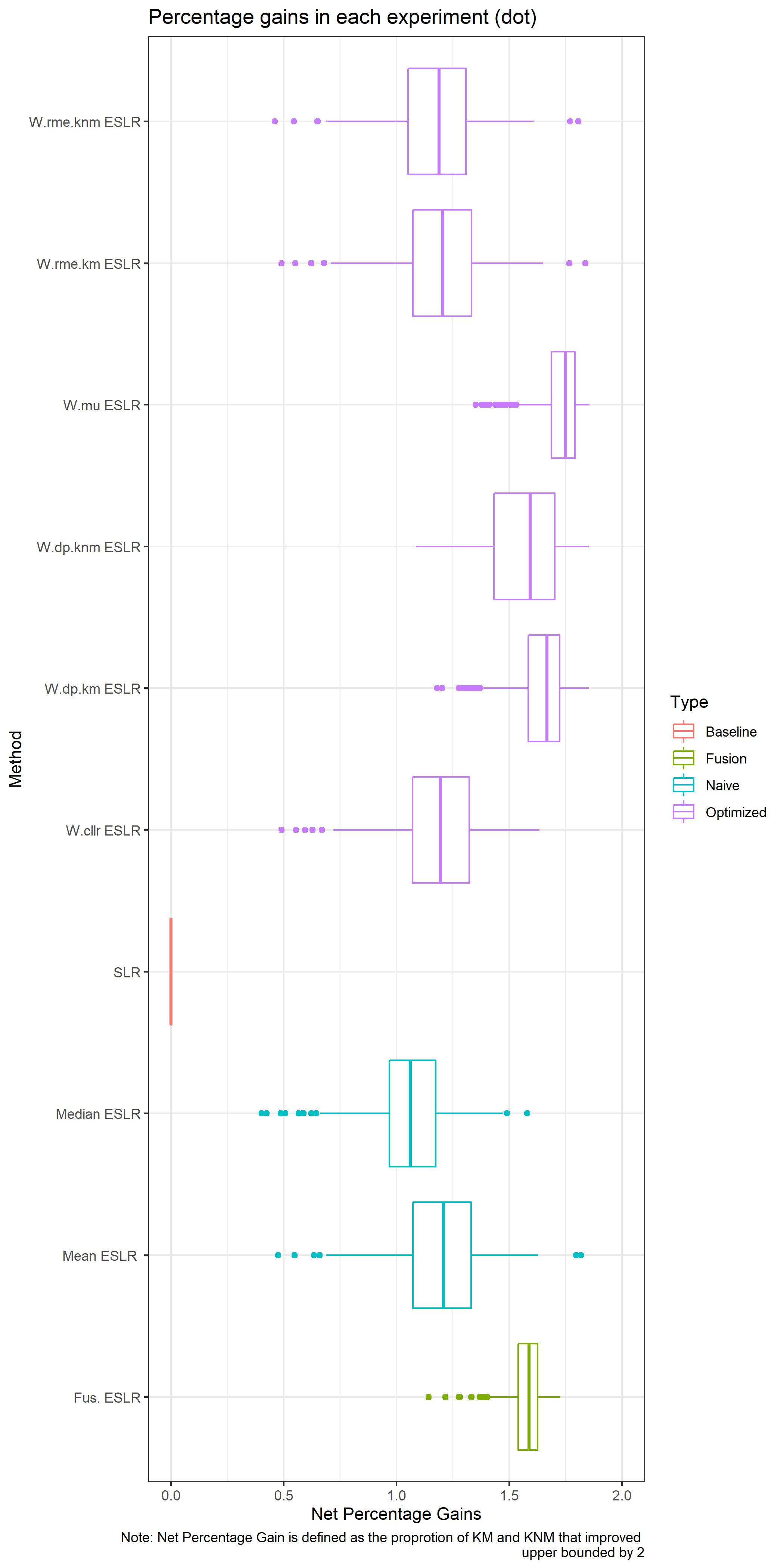
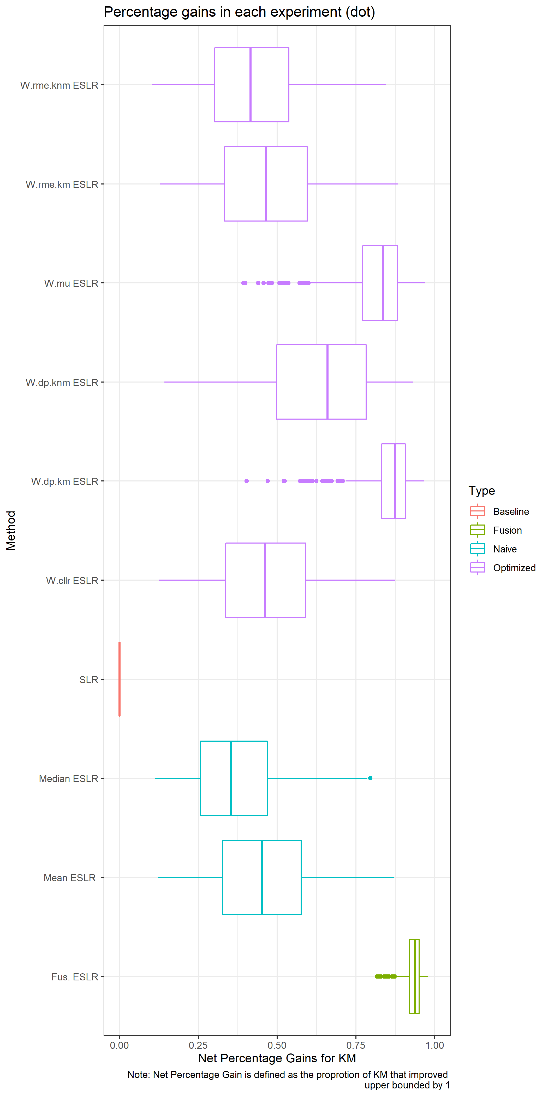
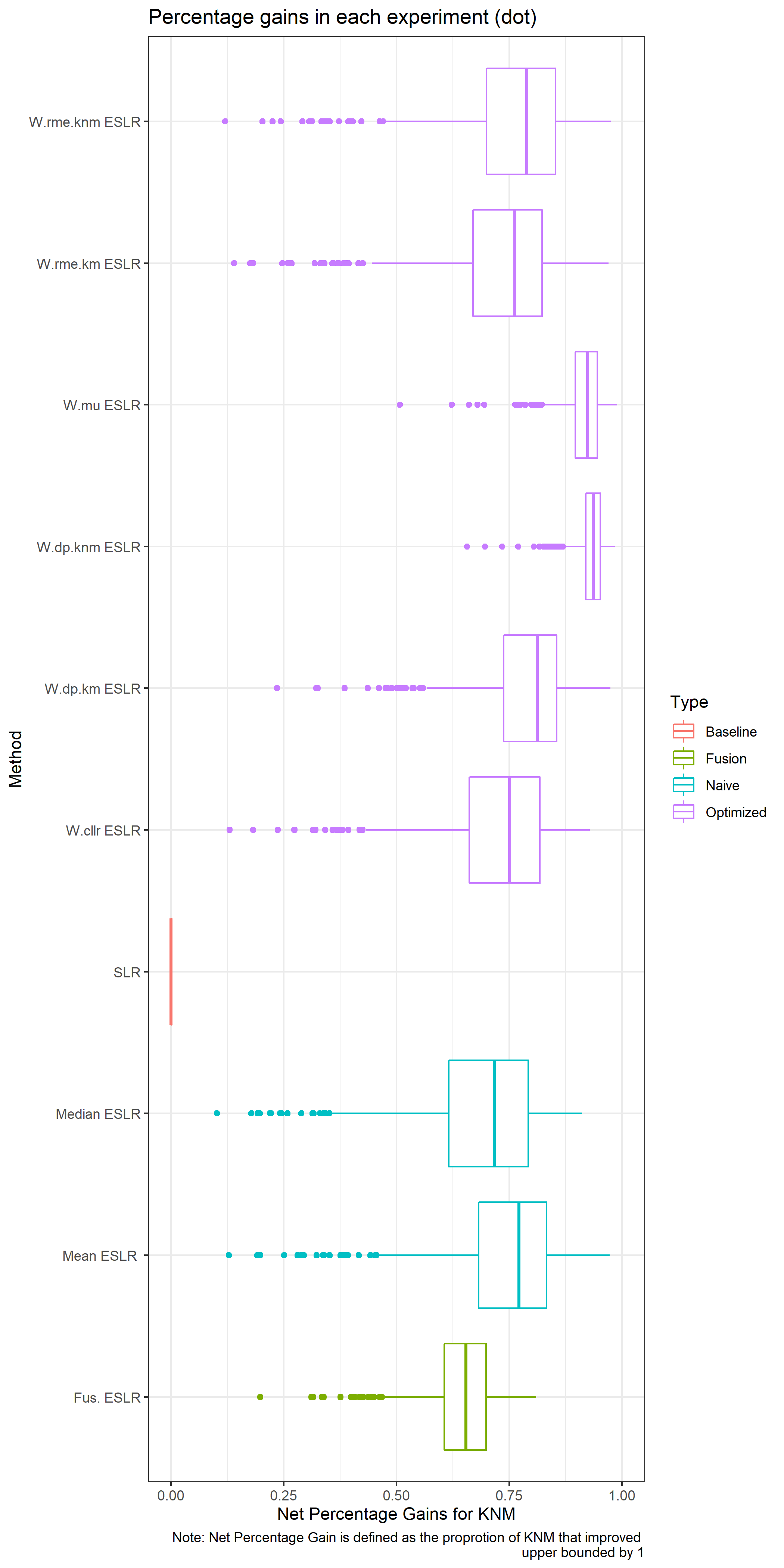
What is the gain with respect to the baseline?
We consider the difference meaning \(ESLR-SLR\).
In the case of KM we would expect to see a positive difference, meaning we provide stronger results for KM.
In the case of KNM we would expect to see a negative difference, meaning we provide stronger results for KNM.
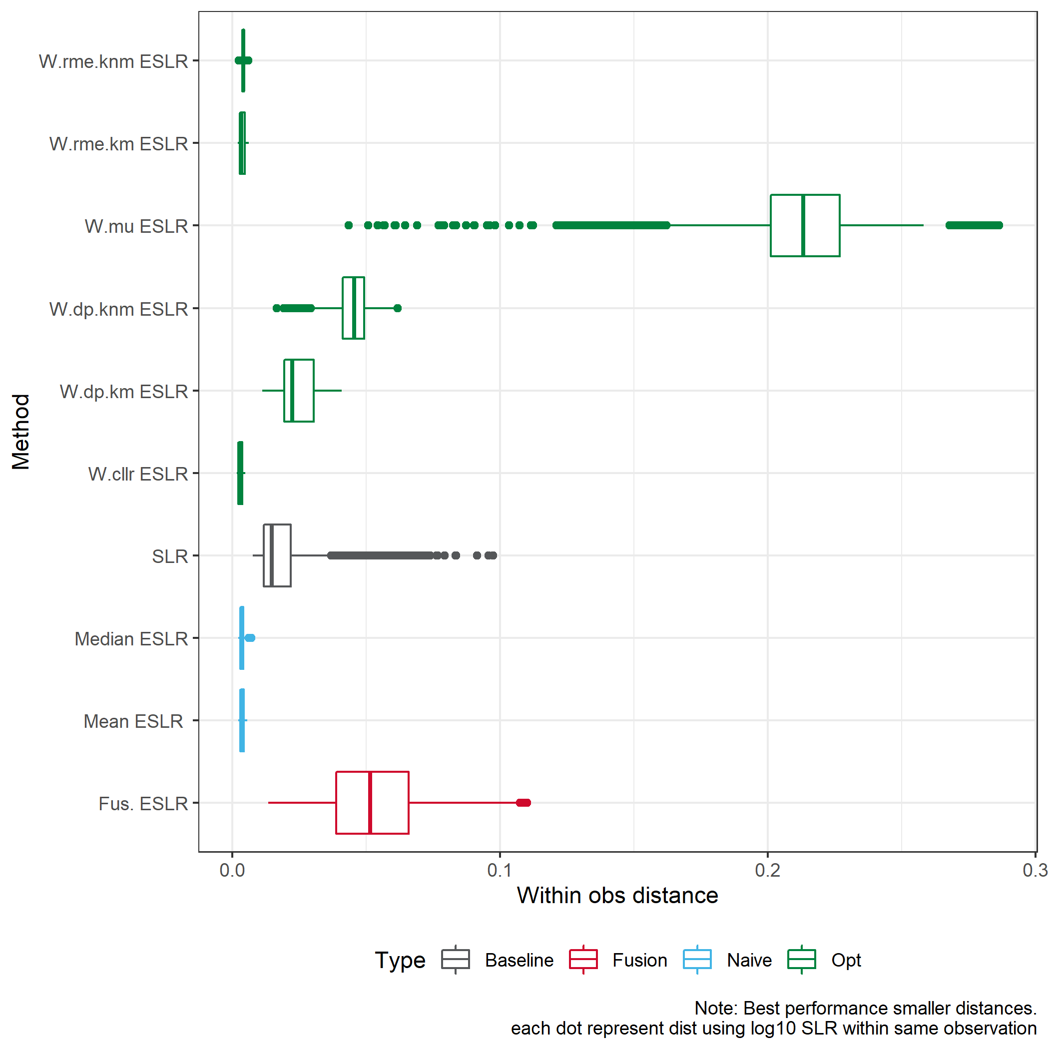
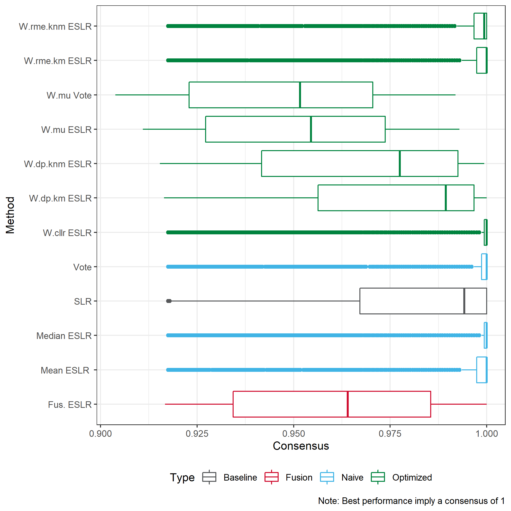
How reliable are the methods. If the training- estimation data is altered, would the conclusions change?
From Experiment 2 we could consider distance metric or a consensus measurement between same observation in the validation set.
We consider the Euclidean distance for log10 SLRs
We consider a consensus measure.
