Chapter 7 Shoes

7.1 Introduction to Footwear Evidence

7.1.1 What is footwear evidence?

Footwear evidence usually refers to imprints made by shoes in some medium. These imprints can either be 2D (e.g. a shoeprint made of dust or blood on a tile floor) or 3D (e.g. a shoeprint made in mud or snow). Less commonly, footwear evidence may also refer to shoes themselves. For example, a woman’s body was found with boots that had scuff marks on the side that prosecutors claimed to be evidence of her body being dragged across the length of her ex-husband’s driveway. However, we will focus on shoeprints rather than shoes themselves.

7.1.2 How footwear evidence is gathered

7.1.2.1 Photography (2D and 3D)

Photographs are usually the first step in the collection of footwear evidence because photography does not risk damaging the evidence. The photographer makes use of a DSLR camera with ideally a 50 mm prime lens (or a zoom lens where the lens is set between 35 and 50 mm), around f/8, and an ISO of around 400. (Keeping the focal length between 35 and 50 mm reduces the distortion.)

In order to reduce shakiness and maintain a view parallel to the ground, it’s essential to use a tripod and some way of ensuring the lens of the camera is perpendicular to the ground. To properly light the shoeprint, an external flash placed at an oblique angle is used. Usually at least 4 pictures are taken (with the flash being placed above, to the right, below, and to the left of the camera, respectively for each of the 4 shots). A remote shutter release is not strictly essential but does reduce shakiness and speeds the process up.

Other than the shoeprint itself, an L scale should be placed at the same level as the bottom part of the impression. This scale will later be used to size and adjust the perspective of the shoeprint. This is easy for 2D impressions but may require additional work for 3D impressions. For example, if there’s a 1-inch deep impression made in mud, you must dig a 1-inch deep area around the impression to place the L scale. A direction indicator should also be placed near the impression. (Often, this indicates north, but it can also indicate the direction to the area the body was found, or in the case of a vertical footprint on a wall, it could indicate “up.”) The L scale, footprint, and direction indicator should fill the photo as much as possible; leave as little empty space as possible so that as much detail of the shoeprint is captured as possible.

7.1.2.2 Gel lifter & electrostatic dust print lifter (2D)

Different crime labs prefer different collection methods. Again, photography is recommended first because the shoeprint may be damaged in the process of attempting to do the lift.

Dust or powder impressions can be found on various types of surface at a crime scene where they may be wet or dried. Such impressions can sometimes be detected with the naked eye, but they can be detected much more easily with oblique light. They can then be collected with a gel lifter or an electrostatic dust print lifter (EDPL).

Gelatin lifter is made of a black gel layer on a flexible woven surface. Once it is placed on the impression, the dust and powder particles forming the impression stick to the gel so that the impression is collected on the lifter. There has been some research on the method for placing and lifting the gel so as not to distort the evidence.

EDPL operates by creating static electricity on a plastic film placed on the impression, and attracting the fine particles onto the film. As a relatively small portion of dust is taken from the impression by EDPL, and the rest is preserved, it is regarded as to be “non-destructive,” so it is recommended to be applied before gel lifters are used. On the other hand, EDPL works well on loose dry particles, but not on wet substrates while gel lifters are generally applicable for both.

Both lifts are easily damaged, though the electrostatic lift seems to be moreso. Because of this, the lifts should be photographed as soon as possible after collection.

Note that online sources (e.g. Guide for Lifting Footwear and Tire Impression Evidence (03/2007)) also mention adhesive lifters, but 1) there isn’t much easily accessible information online about how they are used, and 2) the speaker of the Footwear and Tire Impression Collection Techniques workshop, Heather Connor, said that adhesive lifters are not recommended for evidence collection.

7.1.2.3 Casts (3D)

Casting is used for 3D shoe impressions (e.g. in mud or snow). Different materials are used for different mediums and in different regions. For example, Alicia Wilcox remarked that while she uses dental stone in snow (in Maine), she knows someone in Alaska who uses sulfur due to the difference in the water content of the snow.

The cast may need to be left about 30 minutes (time varying with the weather conditions and the cast mixture) before removing it from the shoeprint, and 24 hours before it hardens enough to clean the cast itself of dirt or other debris. In order to use the cast to compare, the cast may be used to create a 2D shoeprint like the known shoe techniques described below.

7.1.2.4 Known shoe

All the above techniques are used for the “questioned shoeprint,” e.g. the shoeprint present at the crime scene. However, we are also interested in the “known shoe,” e.g. the shoe of a person of interest and shoes collected for research purposes.

Usually, the known shoes themselves as well as shoeprints made with the shoes are used. This can be done in a variety of ways. Of course, the methods listed above can be used as well.

• Everspry Outsole Scanner (EverOS; 2D)

• Everlast Shoeprint Scanner (EverLSS 360)

• 3D scanners

• Inkless technology (Sole Print from BVDA, Identicator LE-25 from Evident, Sole print inkless Shoe Print Kit from Arrowhead Forensics, EZID System from Sirchie) cf. A lecturer at 2021 IAI said Identicator LE-25 has been popularly used.

• Fingerprint powder on white adhesive with cover sheet

• Fingerprint powder and roller transport film (Kodak roller transport cleanup film #4955; Roller transport clean up film available from Safco Dental Supply)

• Powdered impression on gel lifts

• Ink on clear wet media film (more of a method for tires)

• Greasy mark, paper & fingerprint powder

• Forensic photo table with lighting techniques

• Shoe itself

7.1.3 How footwear examination is done now

Footwear examination is done by footwear examiners, who are usually separate from the people who collect the evidence at the crime scene, i.e. crime scene investigators. They may work in a different department or even at a separate crime lab that receives evidence from many different police departments.

Other than side by side comparisons of the questioned shoeprint and the known shoe/shoeprint, examiners also use overlay with transparencies.

Examiners use Photoshop to adjust the perspective of the object in photos, brightness, contrast and total range, and to calibrate the size using the L scale in the photo. Processed photos are then compared on screen by overlaying the questioned and known image and coloring the two images differently. The transparency of images can be adjusted in Photoshop, so one of the images can be converted to a relatively transparent image when it is overlaid over the other to see the similarity and differences. Printed images are likely to have lower resolution, and thus lose the detailed information.

7.1.3.1 What do examiners look for?

7.1.3.1.1 Class characteristics

Class characteristics are size, physical shape (left vs. right), outsole design, and manufacturing variables. Some people also classify “general wear” under class characteristics as well. Most footwear comparisons are class comparisons. In fact, William Bodziak claimed that 90-95% of comparisons are class comparisons.

Size is more complicated than it might seem. The physical size of the outsole often differs from the labeled/marketed shoe size. This is because the same outsole can be used for more than one shoe size; for example, the same outsole could be used for sizes 6-8. Usually, only physical sizing may be determined, unless there is an imprint of the labeled shoe size. Footwear examiners and researchers should thus be wary of saying that a shoeprint is a certain size.

Design is more or less self-explanatory. A couple things that footwear examiners pay attention to is the number of a certain element (e.g. the number of circles lining the edge of the outsole) and where an element intersects with another element (e.g. what part of the zig zag pattern intersects with the edge of the shoe). Also note how size and design can be related: some elements of the shoe design could increase in size with the shoe while other elements only increase in number.

The way the shoe was manufactured can also give the examiner information. Some shoes, mostly flip-flops and sandals, are cut; the overall pattern is printed out and then the outsole is cut out from that sheet, leading to a more random distribution of the pattern. Other shoes are made from molds. (William Bodziak said 99% are made from molded outsoles, a few of which are then trimmed to their final dimensions.) Nowadays molds are usually created with Computer Aided Design - Computer Aided Manufacture (CAD-CAM), which result in identical molds. Hand-milled molds used to be more common, and each mold was different. Regardless, after the mold is created, texture is added to each mold. Texture is usually created either with hand-struck stippling or acid etching, both of which tend to result in some uniqueness in position/pattern, allowing the examiner to identify that two shoes were made from the same/different mold if there is enough texture detail present. Note, however, that Nike Air Force 1s and similar Nike models are an exception; a pre-molded insert is used for each shoe size for the star texture in the toe and heel, so, for those Nike designs only, same size molds will share identical texture in the toe and heel area. (The texture on the other parts of the outsoles will still differ mold to mold.)

General wear refers to the wearing away of some elements of the shoe (e.g. the heel area). Examiners can compare the amount and location of wear between two shoes/shoeprints. Note, however, that wear changes over time, and thus the examiner must be aware of when the crime took place and when the shoe of the person of interest was collected.

7.1.3.1.2 Randomly Acquired Characteristics (RACs)

Unless a shoe design is incredibly rare, class characteristics do not allow an examiner to make an identification conclusion. That’s where randomly acquired characteristics (RACs) come in. RACs include cuts/scratches, tears, holes, abrasions, stone holds, additional debris, and extreme wear. Asymmetric RACs (e.g. scratch) are considered more unique than symmetric ones (e.g. circle) because a different position of the RAC is identifiable as different. Examiners use multiple RACs to make an identification conclusion.

The Schallamach pattern is a ridge-like design produced by the erosion of the outsole in contact with a surface. Footwear examiners compare the Schallamach pattern to a fingerprint. Because the pattern is so shallow, it can change in 6 hours of wear according to Alicia Wilcox.

7.1.4 Common shoe designs

According to Jon Byrd, the most common shoe design in crime scenes (and the most sold shoe in the U.S.) is the Nike Air Force 1. In contrast, Kent Timothy said he mostly sees Vans and Converse shoes. The prevalence of a given shoe design thus varies across the U.S. However, all three of these shoe designs are common enough that most, if not all, of the footwear workshops focused on distinguishing different designs/molds of each of these three designs. Also note that the most popular shoe designs often also have knockoff or counterfeit versions.

7.1.5 How often is footwear evidence used?

Footwear evidence is very common at the scene of the crime. As one speaker at the conference noted, criminals can use gloves to cover their hands but often don’t take steps to cover their shoes (pun unintended). However, it seems that footwear evidence is not actually often used in the U.S. (though it may be used more often in other countries such as Great Britain).

How did I come to this conclusion? At the Footwear Comparisons for the Experienced Examiner workshop, Alicia Wilcox made the remark that there are few footwear examiners (and especially experienced footwear examiners) in the U.S. That advanced workshop only had ~12 participants in comparison to the Basic Footwear Comparisons which had many more (maybe ~30), the latter having participants who were inexperienced footwear examiners as well as prospective footwear examiners (some who may have been uncertain about becoming a footwear examiner). (These numbers are rough estimates as I didn’t think to record them at the time. However, I felt that the former workshop was less than a third full, and the latter was almost completely full.) Additionally, in all three footwear workshops I attended, the speakers made remarks about footwear rarely being collected. These two factors may be a chicken and egg story.

There are three reasons for the low usage of footwear evidence that I can think of and/or have been referenced by the speakers at the workshops.

First is that collecting footwear evidence takes time. Crime scene investigators are often on a time crunch which varies with the severity of the crime. For example, they may be expected to finish collecting all evidence at a burglary in 30 minutes but given more leeway for a murder.

Second is that footwear examiners may need a long time (even weeks) to fully analyze a pair of shoeprints.

Third is that footwear examiners often don’t come to a decisive conclusion (i.e. exclusion or identification) and instead conclude something weaker (e.g. association of class characteristics). (See SWGTREAD for standards on footwear conclusions.) Investigators may become frustrated at what they view as non-answers.

7.1.6 What questions are open/interesting?

Note that footwear examination is currently purely qualitative. How could we apply a quantitative/statistical approach?

One way is to find out how accurate current (or proposed) practices are. These are known as black box studies. Although we do not know exactly how examiners come up with their answers, we can measure false positive rates, false negative rates, etc. There are some issues that may arise from such studies. For example, these studies are often not done in a way that mimics casework, and examiners are aware it is a “test” rather than “real” and thus may change their behavior; however, it can be argued that such a study will still give an approximate accuracy which is better than nothing, and moreover it is much more difficult to conduct a “more realistic” study. Another issue is how to deal with “inconclusives.” In the case of footwear evidence, SWGTREAD’s proposed standards for footwear conclusions have two “conclusive” answers (i.e. exclusion and identification) and five “inconclusive” answers (i.e. lacks sufficient detail, indications of non-association, limited association of class characteristics, association of class characteristics, high degree of association). How do we treat these inconclusive answers in our calculations of accuracy?

Other questions we can ask are lower-level. For instance, since we often can only identify class characteristics, we may want to ask how common a shoe of some size and design is. While we may be able to obtain sales data, how does that sales data correspond to the shoes people wear in real life? Does the frequency of a particular shoe change depending on the geographical region, time of year, day of the week, whether the area is urban vs rural, etc? Since thousands of new designs are released every year, this exact question of frequency of a particular size/design may be infeasible to answer. Instead, we may want to ask a more general question such as the frequency of a flower design. Vanderplas, Stack, UNL; Stone, Fales, ISU are currently working on a project to answer this question. They’ve built a scanner that can be walked across, and several scanners will be installed across Ames in high-traffic areas. The goal is to collect many images of shoe soles, identify different elements in the soles, and compute the frequency of different elements.

RACs are also a key part of footwear evidence analysis. Since RACs are often used for identification, we’d like to know how common/rare different RACs and their locations are. Also, are footwear examiners good at identifying RACs? A small study was done by Stern, Katz, Kaplan-Damary, UCI. A member of the audience at Alicia Carriquiry’s talk at IAI made some suggestions for further studies: 1) ground truth could be determined by taking a scan of a new shoe and comparing it to the shoe after it’s worn; 2) the identification of RACs should be done by footwear examiners rather than students trained by footwear examiners; and 3) the examiners should also be provided with the actual shoe instead of just the shoeprint.

Finally, can we make a directly quantitative comparison between two pieces of footwear evidence? For example, can we create a similarity score that distinguishes between matches and non-matches? Park, Carriquiry, Lee, Han, ISU have worked and/or are working on quantifying the similarity between 2D shoeprint scans.

There are so many other interesting questions we are interested in. For example, in what way and how much do shoes deform when walking, running, etc in comparison to stepping straight on and off? How does weight and/or height affect a person’s shoeprint? How do jurors view/understand the SWGTREAD conclusions?

Many of these questions are complicated by the variety of footwear evidence. Footwear evidence can be a whole shoeprint or a partial one, 2D or 3D, be made in different matrix/substrate conditions, made while running/walking/etc., the known shoe could be collected months later or immediately, etc. In any given study, we must make a choice about the type of footwear evidence we consider.

See the OSAC Footwear and Tire Committee for more research areas.

7.1.7 Current work

[to be filled in by different project members]

7.2 Longitudinal Shoe Study

Github repository

7.2.1 Paper describing the database

Paper subdirectory of Github repository

Goal:

• Describe experiment
• Describe database function
• Publicize data for analysis by others in the community

Accompanied by Figshare upload of static data sets (grouped by type).

Data Analysis Tools

• Working with the EBImage package - very fast processing of images

ShoeScrubR package

Cleaning methods for the Longitudinal data are contained in the ShoeScrubR package. The package includes (as of 2019-10-17) a complete set of tests to guard against regressions (100% test coverage!) and uses continuous integration to ensure that the installation process is also monitored.

The ShoeScrubR package also includes logging of all image-in image-out operations using attributes - each time a transformation is performed, the transformation and the parameters are appended to the running operations log. This should make it possible to track the provenance of an object through the set of transformations (and potentially un-do them in some cases).

Film and Powder Images

The images are challenging to do basic statistical analysis on because the shoe print is made up of tiny particles (e.g. it is not a solid object), and there are areas of smudged particles outside the image (fingerprints, etc.) that can be hard to automatically remove. In addition, the film backing has subtle variations in color.

The prints are not rotationally aligned, that is, they are taken at a variety of angles (usually \(\pm 15^\circ\) from vertical) which vary due to individual differences in walking style, the orientation of the film, and changes in experimental protocol.

Experimental protocol changes included resolution changes for the scans over time: the resolution of the last set of images is about 2 times higher than the resolution of the first 3 check-ins worth of images. Thus, parameters need to be automatically selected based on the resolution of the image.

The initial use of templates to clean up the image requires addressing the alignment of the print and the template. As this experiment contains 8 total shoe model and size combinations, it is possible to create a template for each shoe model and use that template to isolate the region of the image which contains a set of features most likely to be a shoe (rather than random noise).

Solving the template problem by aligning the mask and template yields an additional benefit: the resulting cleaned up image is roughly aligned relative to the template and, presumably, to other images.

Rough Alignment of Template Mask and Image: Clean images, do a rough alignment between the image and the corresponding shoe mask (per model and size).

1. Rotationally align image and mask using principal components on the non-background pixels in the image

2. Gross align the non-background pixels in the image and mask

   • Use a “mask-ified” version of the shoe print that encloses most of the shoe region in a single region (see below for explanation)

   • Default to trimming the actual print by 5% on each dimension to minimize the effect of page borders and creases

   • Alignment method options:

     • center of mass - this fails if a print does not account for the whole shoe
     • center of narrowest width - ideally, this is approximately the arch of the shoe.
       This works better than center of mass in most cases, but occasionally computation fails because it relies on finding a local minimum near the center of the image; if the derivative calculation fails, the algorithm falls back to the center of narrowest width.

3. Pad the image and mask so that the centers are aligned and the image and mask are the same size

4. Set any pixels outside the mask to background

Before:

After:

These steps are wrapped into the rough_align function in the ShoeScrubR package.

Cleaning the image and exaggerating into a mask

In several of the methods applied to this data, it has been useful to have an exaggerated version of the image to function as a mask - this exaggerated image has a center of mass similar to the actual mask, for instance.

Creating this mask requires parameter tuning (done the old way); a new method was developed in order to reduce the number of parameters which depended on image resolution and other similar items.

In the old method, there were several parameters necessary - gaussian blur diameter for image cleaning, threshold for binarization, gaussian blur diameter for mask creation, threshold for image cleaning, diameter for opening the mask, diameter for closing the mask.

The new steps are as follows:

1. Use the EM algorithm to cluster the intensities of the points into three normally distributed categories: signal, intermediate, and background. The normality assumption is highly questionable, but the method works pretty well. Use the calculated pdf values for each point to construct a likelihood ratio of P(signal)/P(intermediate + background). Binarize based on the value of this likelihood ratio - if it’s over 10, the pixel is signal.
   • Each shoe is shown in three separate images, corresponding to the pdf value for each point based on the EM algorithm clustering distribution fitted values. White pixels are highly likely to belong to the group in question - signal, intermediate, and noise.
     
     
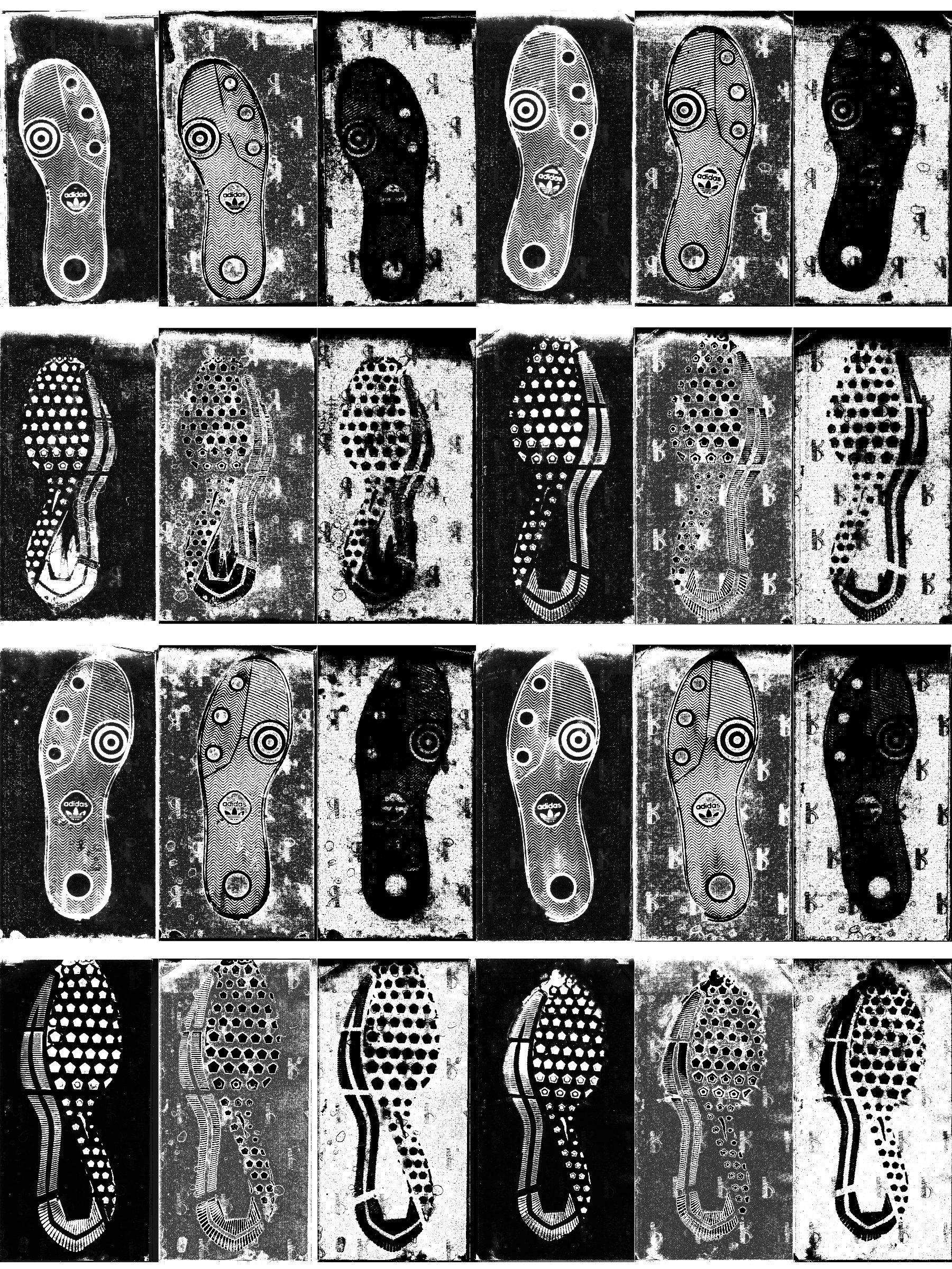
   • Binarized versions of each shoe
     
2. The binarized image from the EM algorithm is cleaned slightly using parameters that should be robust to different ppi images (diameters < 10 pixels) - this gets rid of speckling induced by the EM segmentation.
   • Initial cleaning - dilation and erosion at very small pixel values
     
   • Labeling disjoint regions (different colors indicate different regions)
   • Removing any blobs which are in the 50px square corner region and which do not involve more than 10% of the image.
     
     At this point we can use the mask to clean the image:
     
3. The binarized image is exaggerated using parameters which depend only on the size of the image. In general, size \(s\) here is the square root of the number of pixels in the image, that is, the side length of the image if it were square.
   • A gaussian blur is applied to the image (diameter \(s\)/50)
     
   • Any pixel intensity less than the median is determined to be shoe
     
   • All disjoint regions are labeled
     
   • The largest region is selected as the best mask for the shoe
   • Some cleaning is done to this mask - any holes are filled in and then it is opened by a diameter of approximately \(s\)/5 (must be odd)
     

At this point we can use the mask to get a “clean” image:

And proceed with the alignment as normal:

Aligning each image to the template corresponding to the shoe model and size provides a good first step towards aligning the images to one another, but additional work is necessary in order to ensure that we can compare two images from the same shoe (or two images from different shoes).

Fine Alignment of two images using RNiftyReg

The RNiftyReg package is intended for alignment of brain scans and other MRI data and uses a symmetric block-matching approach(Modat et al. 2014). It only allows for registration of images up to 2048x2048, though, which means we will have to align images at a lower resolution and then modify the transformation matrix accordingly. One definite positive feature is that it allows for provision of a mask for both the source and target images so that only pixels within the mask are used for alignment.

Affine transformations are a type of image transformation that encompasses translation, resizing, rotation, and skew operations. Affine transformations preserve collinearity and ratios of distances: parallel lines remain parallel after the transformation. A subset of affine transformations are so-called “rigid body” transformations, which only allow translation and rotation.

RNiftyReg allows for linear (rigid-body, affine), and nonlinear transformations, but for the moment, we are only interested in rigid-body transformations - while the shoes may have some slight distortion due to the wearer and kinematics of walking, this is minor and should not interfere too greatly with a gross alignment.

RNiftyReg’s niftyreg.linear function returns a 4x4 transformation matrix describing the composition of multiple image transformation operations. A 3x3 matrix is necessary for 3-dimensional image rotation, resizing, and skew operations; it is then augmented by a row of zeros on the bottom and a column ending with a 1 that describes the x, y, and z translation coordinates. In this way, a 4x4 matrix can represent the composition of all relevant image transformation operations in 3 dimensions. In two dimensions, many of the cells in this matrix are 0.

1	2	3	4
5	6	7	8
9	10	11	12
13	14	15	16

Cells 1, 2, 5, 6 describe the rotation operation; the angle of rotation can be recovered using trigonometry.

Cells 4, 8 describe the translation operation, e.g. the row (4) and column(8) offset from one matrix to another.

For 2D rigid transformations, these are the only cells which matter. Cells 11 and 16 are 1, and 3, 7, 9, 10, 12, 13, 14, 15 are all 0 under these constraints.

In order to use RNiftyReg for registration of the original-size images, we have to scale cells 4 and 8, but the rest of the cells remain unscaled.

Note that EBImage uses what is essentially the transposed version of the matrix used by RNiftyReg, reduced to elements 1, 2, 5, 6, 4, 8 in a 3 row by 2 column matrix.

1	5
2	6
4	8

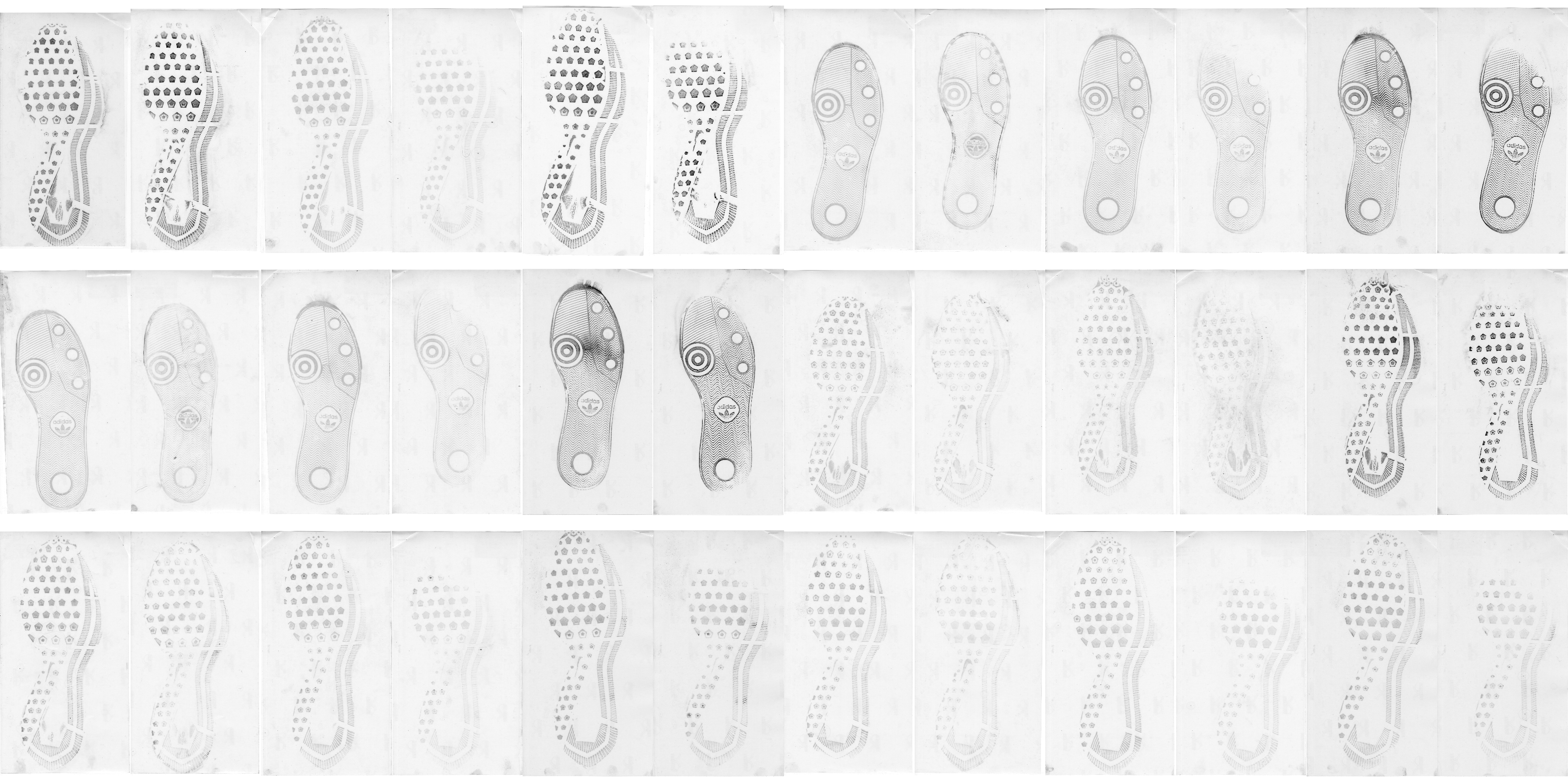
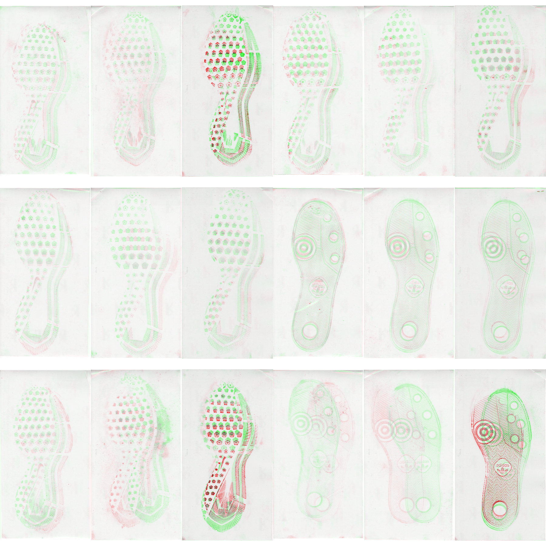
Starting with a set of 6 shoes observed at 3 timepoints each, with 2 different “modes” of print capture, we can align both prints taken on the same date for each shoe.

The original images: (1 and 2 are taken at the same time point, 3 and 4, etc. 1-6 are the same physical shoe over time and so on)

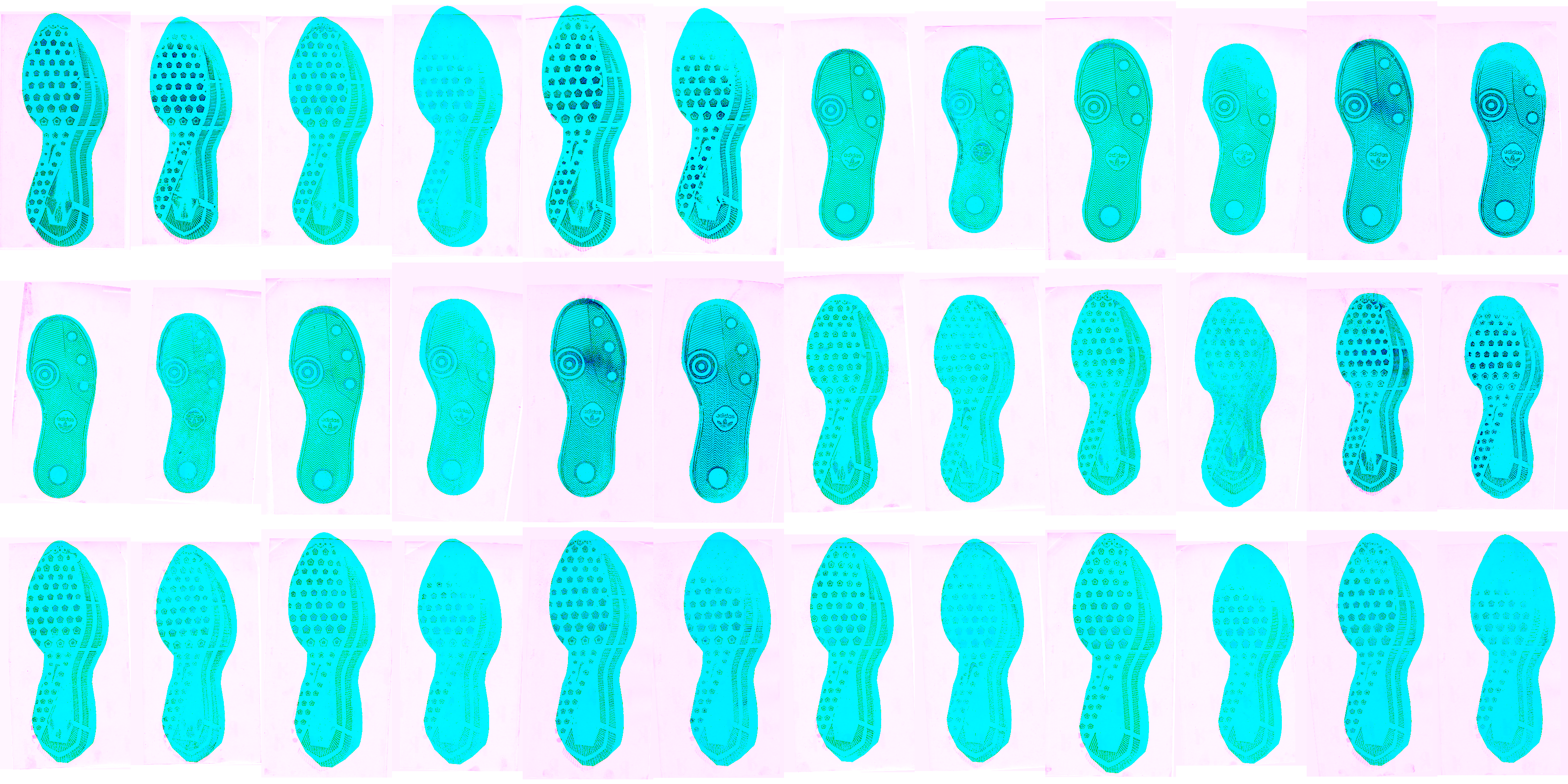
The images are first aligned to masks, which are used to clean the images to reduce noise.

Then reduced-size versions of each image pair are aligned, producing a transformation matrix:

0.9999730	-0.0073485	0	30.48815
0.0073485	0.9999730	0	-10.16105
0.0000000	0.0000000	1	0.00000
0.0000000	0.0000000	0	1.00000

(this is one example)

The coordinates in bold have been scaled according to the size reduction, so that they can be applied to the full-size images.

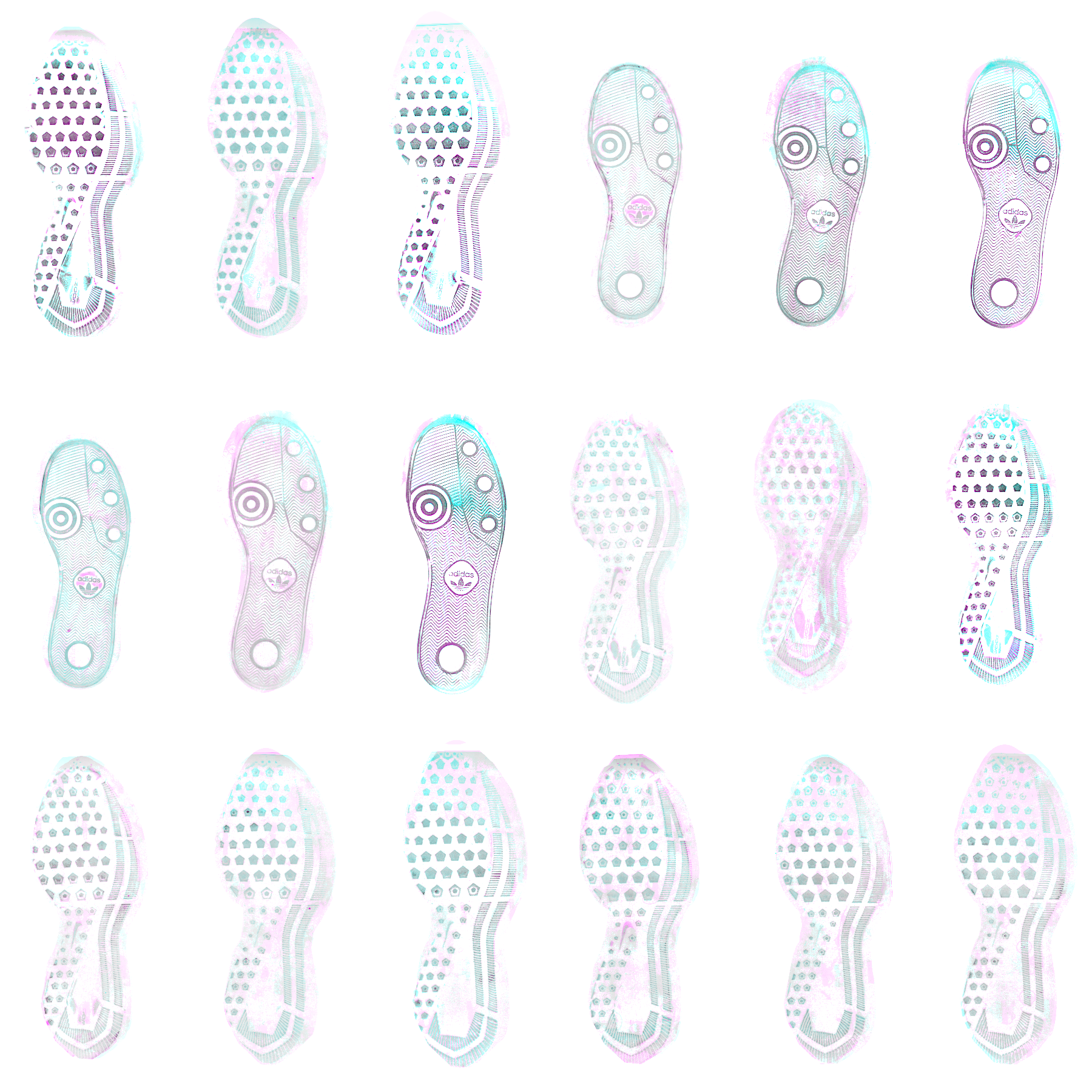
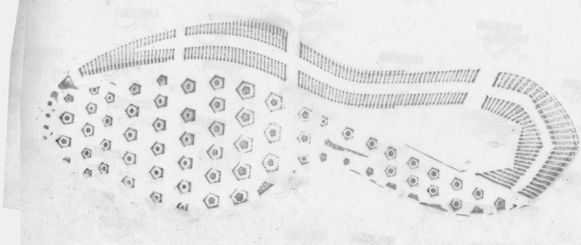
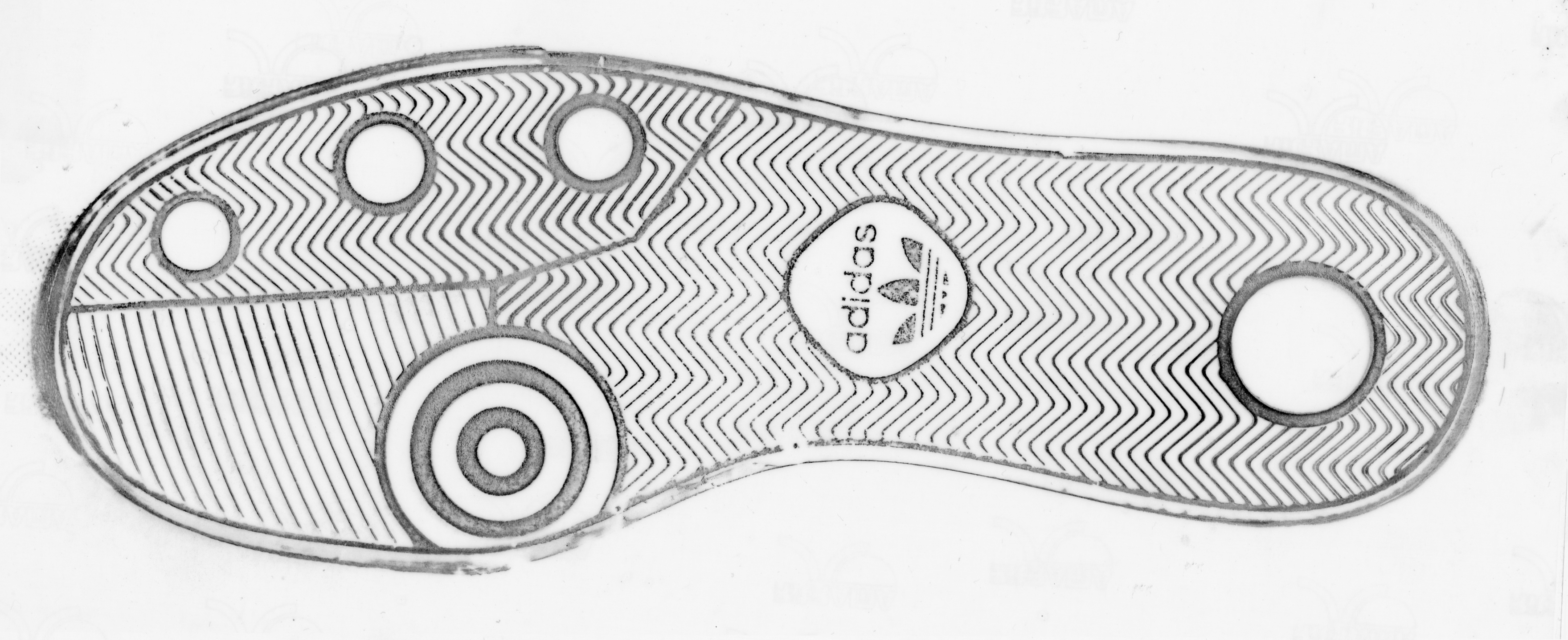
The resulting aligned images are shown above; black pixels are areas where both images agree; pink and blue pixels represent areas found in one image but not the other. Some images which have many bubbles (air between the film and backing) or which contain blurred or double prints do not align accurately; this is really not avoidable with automatic alignment solutions.

The alignment process itself (without any image preprocessing) is extremely fast, about 1s per image pair, and seems to be similar even when image size is increased by a factor of 16. Due to the scaling process and necessary modification of the transformation matrix, the alignments may be off by 1-5 pixels in some cases. This might be handled by aligning a smaller subset of the image at full resolution. Efforts to align sub-images produced less accurate alignments, likely due to the kinematic distortion of the sole during the walking process, resulting in situations where the local alignment estimate is not a good estimate of the global alignment. New attempts to find consensus alignment might include keypoint-based alignment methods, trying to identify the shoe border precisely to align that, and possibly use of Hough transforms to identify specific reproducible features that might serve as global keypoints.

Given how well RNiftyReg works, the next question is whether all of the preprocessing is even necessary.

In the image below, the first row is alignment with the full image, the second is alignment with a binarized version of the output image (so masked + thresholded), and the third is automatically cropped around the mask which is aligned to the image using the rough-align process. The third row maintains most of the information and produces better alignments than the other rows; thus, we can conclude that it’s necessary to combine the preprocessing and rough alignment in order to get the best results from RNiftyReg.

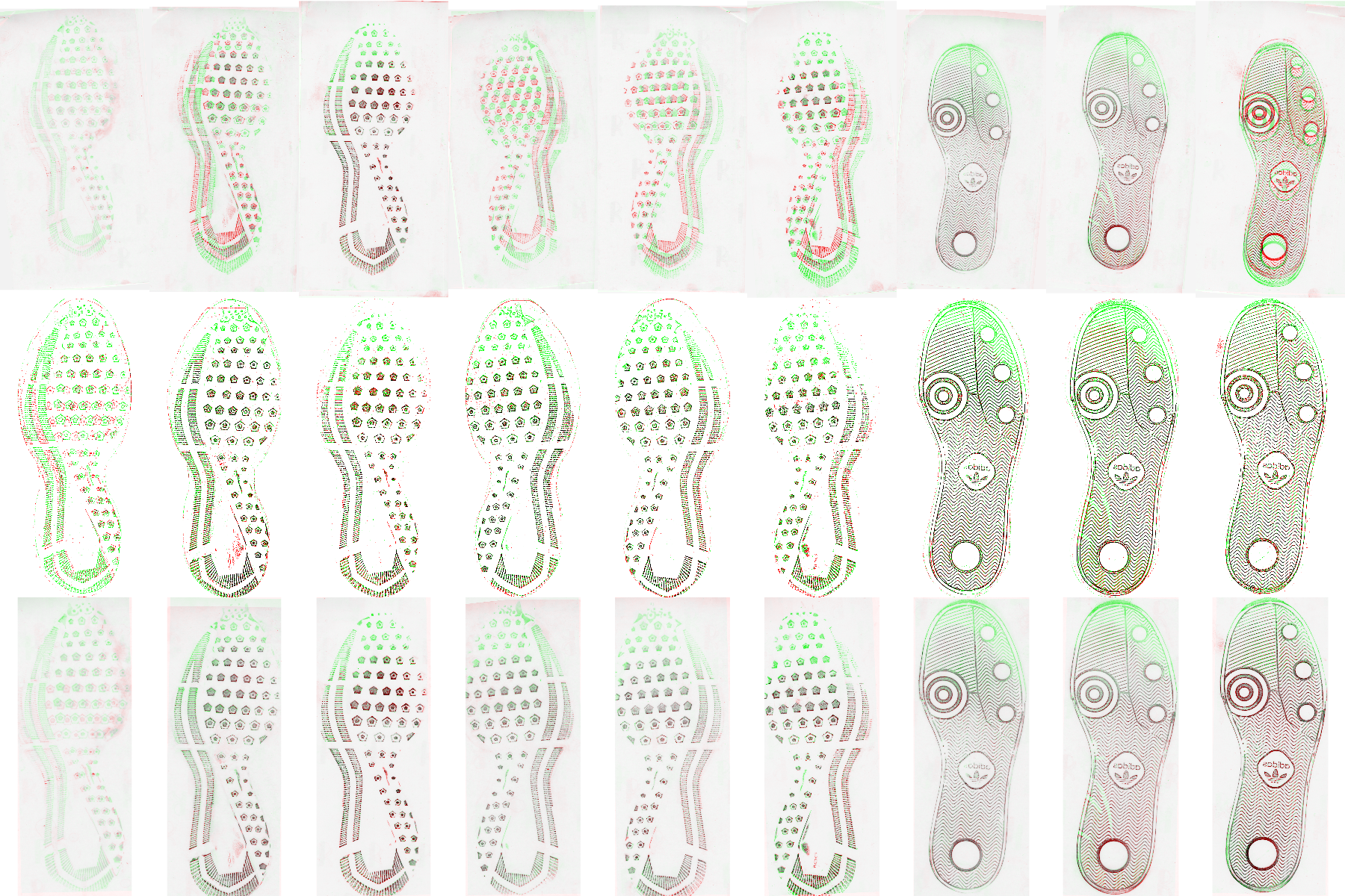
Fine Alignment of two images using FFT

Basic Process:

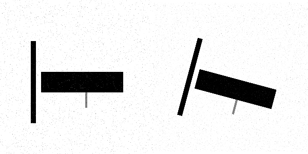
1. Pad images so they’re the same size (Let’s say that \(A\) and \(B\) are the two images)

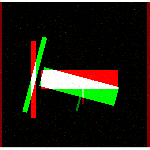
2. Downweight the edges of the images using a Hann function
   This is necessary because Fourier transforms assume images go on forever, so abrupt changes (e.g. edges) don’t work out that well. Computationally, the image is “wrapped” around itself to be considered “infinite”.

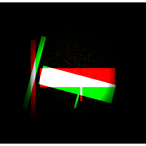
• The strength of the Hann function can be adjusted by a power argument
  

## Error in library(tidyverse): there is no package called 'tidyverse'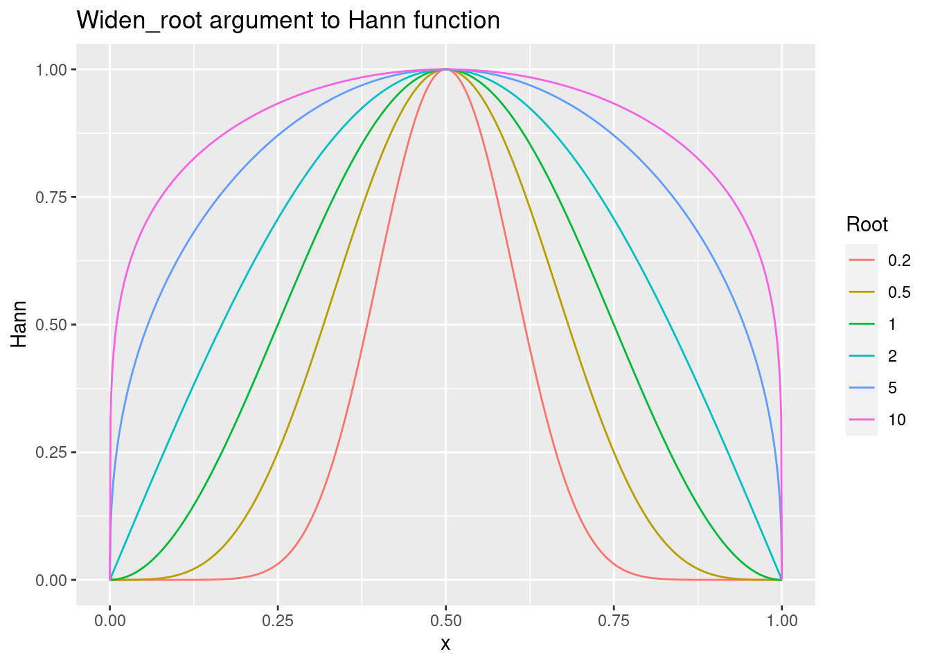

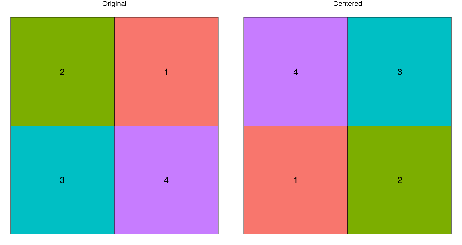
3. Use the Fast Fourier Transform on each image. Center the FFT’d images so that low frequencies are in the center (exchange top left quadrant with bottom right, and top right quadrant with bottom left). Call the FFT’d, centered images \(F(A)\) and \(F(B)\)
   

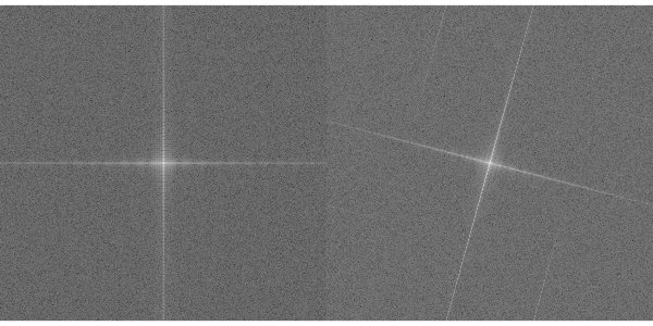
4. Recover the angle between the two images:
   In Fourier space, a rotated image produces the same signal in Fourier space, but rotated. To recover this information, we can use the magnitude of the FFT’d images as a new image. Call these images \(|F(A)|\) and \(|F(B)|\). Then,

   1. Polar transform the image, so that a rotation of the original image is a linear shift of the transformed image (\(P(|F(A)|)\) and \(P(|F(B)|)\)). Apply Hann functions to the polar-transformed images.

b. Use FFT-based alignment (see steps 3, 5) to pick out the $\theta, \rho$ which best align the two polar images

c. Discard $\rho$ and keep $\theta$. Transform the original image (not the FFT'd image) to get $\tilde{B}_\theta$ and recompute the FFT on the rotated image ($F(\tilde{B}_\theta)$).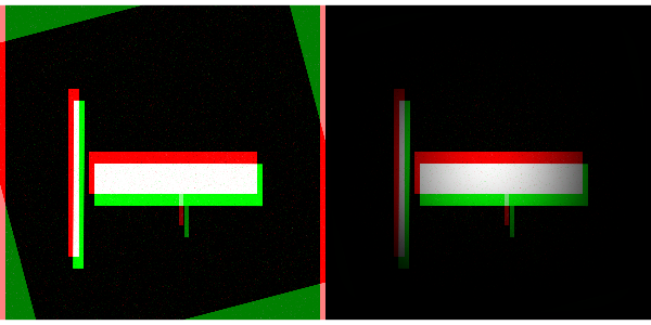     

5. Recover the shift between the two images:

   1. Compute the cross-power spectrum: \(S = F(A) \times F(\tilde{B}_\theta)*\), where \(F(x)*\) is the complex conjugate of \(F(x)\) (e.g. \(a + bi\) becomes \(a - bi\))

   2. Compute the magnitude of the cross-power spectrum: \(|S| = \sqrt{S \times S*}\)

   3. Use (a) and (b) to get the normalized cross power spectrum: \(S/|S|\)

   4. Take the inverse FFT of \(S/|S|\): \(A = F^{-1}(S/|S|)\)

   5. Find the maximum of the \(A\) matrix. The row and column where the maximum is found are the shift to align the two images: \((\Delta x, \Delta y)\).

6. Apply the shift to image \(\tilde{B}_\theta\) to get \(\tilde{B}_{\theta,\Delta x, \Delta y}\).

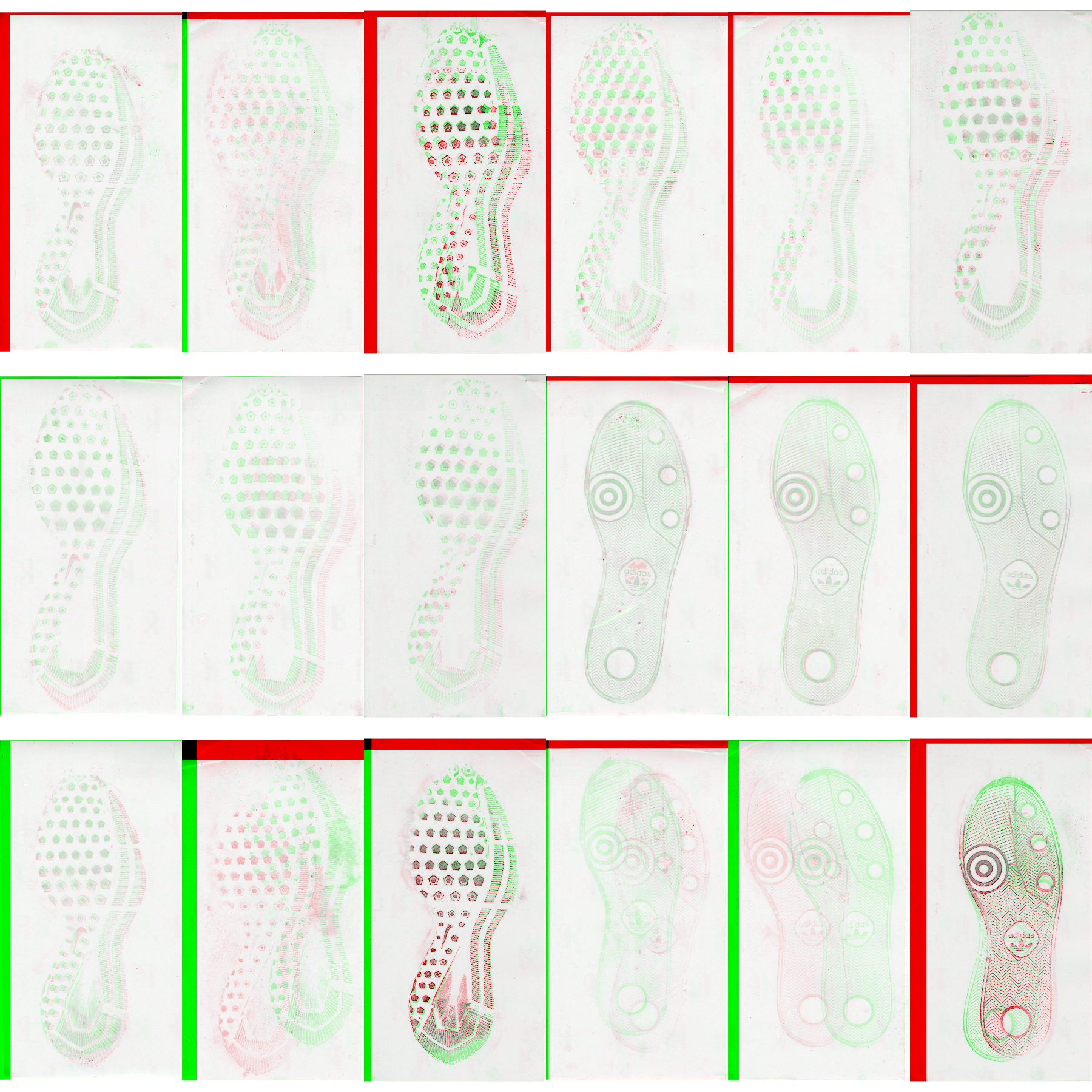
There are some fiddly details (e.g. converting shifts which are most of the image into negative shifts), but FFT-based alignment works pretty well (and pretty quickly) for shoes.

Original Images:

Angle-aligned Images:

FFT-Aligned Result: (still working out the kinks)

Combining information from multiple images

With aligned images, we can then combine the information in each of the two prints taken at the same timepoint to get more reliable images. Because the methodology for acquiring the prints changed from timepoint to timepoint, the analysis of each type of print doesn’t make sense - it is completely conflated with the observation date. However, the multiple prints aren’t wasted, because while each print may be missing information, the combination of both of the prints (when properly aligned) provides a much more reliable assessment of the shoe (and the wear of that shoe at the proper timepoint). There are at least 3 options to combine these images (note that white = 1, black = 0):

• Take the pixel-by-pixel minimum: this keeps all the noise from both images (but there’s relatively little noise in the cropped images, so that may not matter too much). If images are misaligned, this results in a “double” print (or smeared print). This method is also sensitive to the lightness of the print - a complete print would still be ignored if the “dark” part of the print was lighter than the “light” part of the second print.
  
• Take the pixel-by-pixel maximum: this keeps only points which appear strongly in both images (losing a lot of data but also a lot of noise in the process)
  
• Take the pixel-by-pixel mean: This would result in lighter regions where one image has “gaps” but would reduce noise and make it clear where there is less sure information.

Of these options, the first seems like the best, but the last provides some idea of whether the alignment was decent to begin with.

The alignment method seems to fail more frequently when one of the images is very light. It may be advantageous to invest more effort into adaptive histogram normalization.

Alignment Fails:

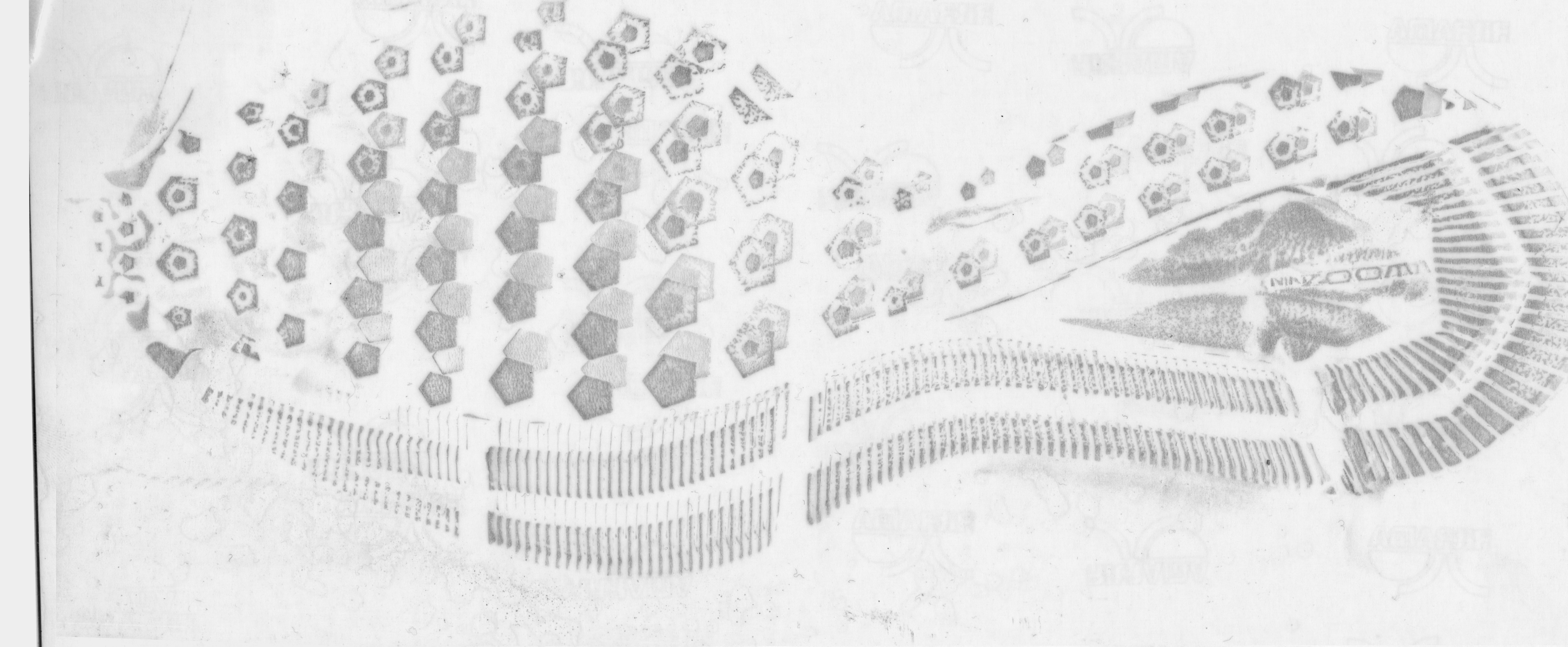
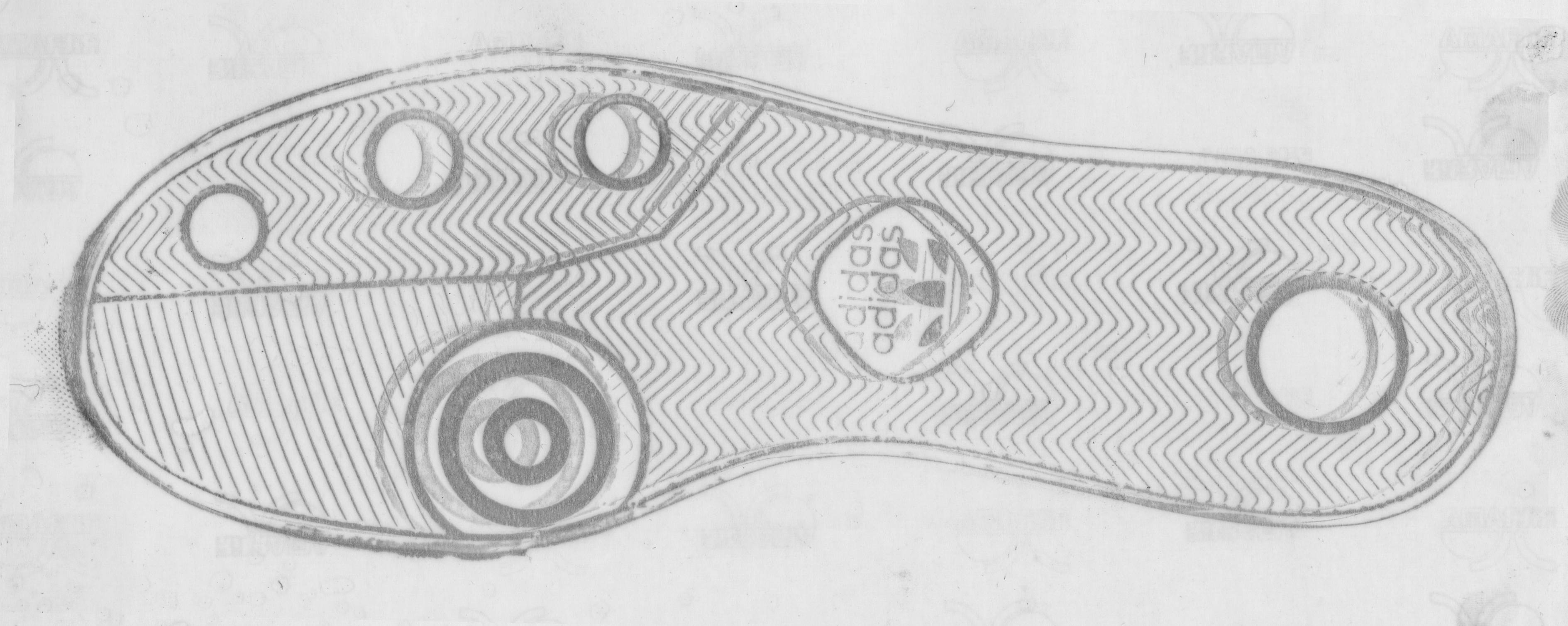
Alignment Success:

Wear Characterization

Ideas:

• average intensity of cleaned image
• length of border/edges detected

7.3 Shoe Scanner - Passive Shoe Recognition

7.3.1 NIJ Grant

Grant scope: Build the shoe scanner, develop an automatic recognition algorithm for geometric design elements, test the scanner in locations around Ames.

7.3.1.1 Hardware

• 2 molds made: Fiber cement held, modified cement is still under testing
• Fiberglass in the ground being hydro-tested
• Big mold - modified concrete, comes out of the mold tomorrow morning (2020-06-02)
• Indoor ramp constructed - can hold 900 lbs safely
• Electronics - waiting on plexiglass - proximity sensors aren’t working in daylight with reg plexiglass. New plexiglass ordered wednesday to diffuse top-light better

7.3.1.2 Software

7.3.1.2.1 Whole-Shoe Object Detection

Project Overview

• Explore the use of RCNNs for whole-shoe object detection

Preliminary results (using ~1000 previously classified images to train and then predict several thousand other images in a semi-supervised approach):

7.3.1.2.2 Restoring Shoe Images

Overview

• Use CNNs to “upsample” manually degraded shoe images (or pairs of ideal and realistic images), restoring as much of the original pattern as possible.

Proof of concept (with awful image scaling to 120x120 px… sorry)

Low light enhancement with CNNs

7.3.2 CoNNOR: Convolutional Neural Network for Outsole Recognition

Project Overview

• Label images of shoes according to geometric classification scheme
• Use convolutional base of pretrained CNN VGG16 and train a new classifier on labeled features
• Eventually, acquire real data passively and use CoNNOR to assess feature similarities and frequencies

Link to submitted Creative Component on CoNNOR

Github repository for paper submitted to Forensic Science International

Exploring new directions:

• Truncate convolutional base and train random forest on features
  • Could replace fully connected layers of neural net as classifier
  • Importance score can filter/reduce the number of features
  • Training the random forest requires too much memory for Bigfoot (CSAFE server), and still takes over two weeks on the HPC. We’re setting this goal aside for now, but could try subsampling the features for a random forest in the future.
• Spatial integration
  • Model is currently set up to take in 256x256 pixels
  • Try taking in full shoe using a sliding window of size 256x256
  • View class predictions spatially
• Fully convolutional networks (FCNs)
  • Unsupervised segmentation to assess current classification scheme
  • Handle whole shoe image of any size (instead of only 256x256 pixel images)

References for CNNs and FCNs

Stack Exchange post explaining patchwise training

“Learning Hierarchical Features for Scene Labeling”: describes an application of multi-scale CNNs and image pyramids

“Pyramid methods in image processing”: classic paper from 1984 explaining pyramid methods

“Fully Convolutional Networks for Semantic Segmentation”

“W-Net: A Deep Model for Fully Unsupervised Image Segmentation”

7.3.2.1 Spatial integration

The overhead costs of going fully convolutional are high; CNN papers are opaque, and many supervised techniques require fully labeled data for semantic segmentation (i.e., label every pixel). Moreover, complex models (for both supervised and unsupervised tequniques) are often only available in Python, and there are a large number of GitHub repositories of mixed quality and reliability. Filtering for quality, understanding code structures, and implementing them on HPC are all enormous tasks on their own.

In the meantime, it is much easier (relatively speaking) to use our existing framework of 256x256 square pixel images, for which we have generated thousands of labeled images and have already trained and improved domain-specific models. Currently, I have code working to automatically crop image borders, chop the image into 256x256 pixels (padding the image when appropriate) and equalize the contrast on the individual images.

Pad the left and top of the image with a pre-specified offset, then chop the image into 256x256 pixel pieces

Equalize the contrast channel for each piece of the image

Use the trained model to predict each piece of the image for each class

Repeat the above process for different cuts of the original image, and aggregate predictions

Updates/In progress:

• Presented on CoNNOR at ISU’s 3-Minute Thesis competition
  • Preliminaries: 8 heats with 10-12 participants each
  • Runner up to a guy making better yogurt
• Implementing semantic segmentation model on HPC
  • Learning HPC structure, command line syntax, using Python in practice
  • Documentation assumes high baseline of knowledge :(
• Improving spatial integration process
  • Remove predictions for blank (and mostly blank) edge images
  • Smooth predictions for overlapping image pieces
    • geom_density2d(), stat_contour(), creating brush overlay with EBImage

Shiny app demo

7.4 Maximum Clique Matching

7.5 Project Tread (formerly Cocoa Powder Citizen Science)

Project Tread, modified from Leverhulme Institute’s Sole Searching, is a developing CSAFE project with the goals of engaging community participation in forensic research and acquiring shoe print data that may be useful in future analyses.

In progress:

• Review procedures and IRB documents written by James
• Volunteers are testing modified procedure (below)
• Be involved in set up of data collection site (through CSSM)
• Develop plan for data analysis and use (to inform procedure modifications)

7.5.0.1 Comparing the procedures

Procedure	Leverhulme	CSAFE (initial)	CSAFE (proposed)
‘Before’ Views	4 per shoe	5 per shoe	2 per shoe
‘Before’ Pictures	1 per view	3 per view	1 per view
Total ‘before’ pics	4 per shoe	15 per shoe	2 per shoe
Paper	Letter (larger)	8.5x11 or 8.5x14	8.5x11 or 8.5x14
Actions	Run, jump, walk	Step, hop	Step, hop
Replicates	6 per action	9 per action	3 per action
‘After’ Pictures	1 pic per rep.	3 pics per rep.	1 pic per rep.
Total # prints	18 per shoe	18 per shoe	6 per shoe
Total # print images	18 per shoe	54 per shoe	6 per shoe
Requested # shoes	Not specified	Both shoes	One, 2nd optional
Total # images taken	22 or 44	138	8 or 16

Recommended procedure modifications:

• Ask for one high-quality image of each shoe angle (‘before’) and print (‘after’), instead of three replicate images of each
  • If Project Tread submission website will be set up like current CSSM system (which takes community submissions for environmental images), intermediate quality control can help filter out bad images
• Only ask for one shoe, and make second shoe optional
  • E.g., always ask for left shoe, and make right shoe optional
• Ask for 3 replicates per shoe instead of 6-9
  • Longitudinal shoe study only uses 2-3 replicates per shoe
• Make written instructions clearer, close loopholes

7.5.1 Pilot procedure testing

Feedback from pilot testing:

• Materials
  • Used 1/4 - 1/2 tsp of cocoa powder, not a “dime-size””
  • Test/specify cocoa powder vs hot chocolate powder
• Procedure
  • Sift cocoa powder onto paper (brushing damages print)
  • More pictures of what things should look like
  • Fewer “before” pictures: bottom and side only
  • Mention won’t see oil if done correctly
  • Don’t stack completed prints until after imaging/scanning
• Analysis
  • Use printable scale/ruler for later alignment of images
  • QR code (like handwriting study) to identify action/replicate/meta info
  • Collect shoe demographics (brand, size, measurements of length/width)
  • Get “mask” by tracing around shoe

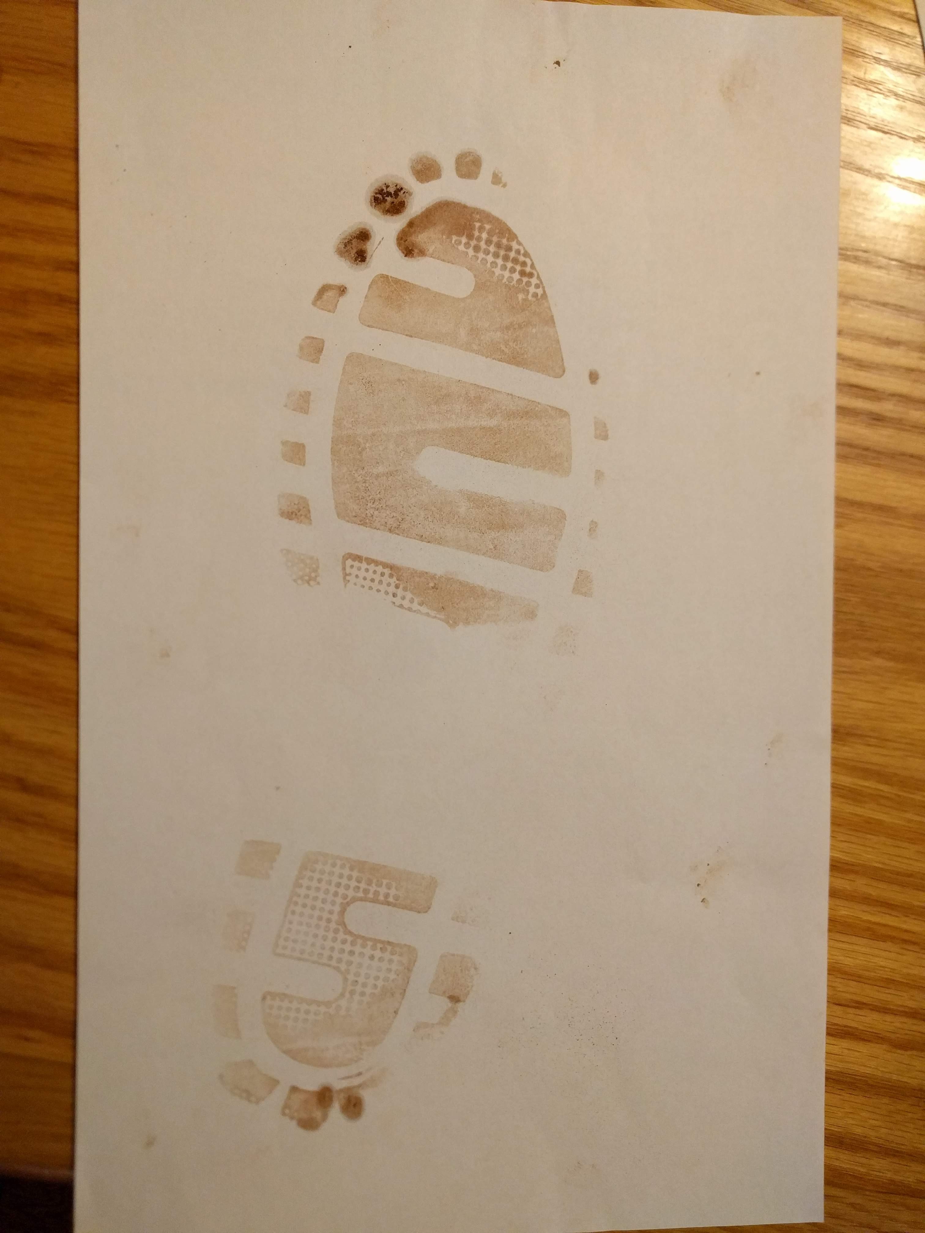
A few images from pilot testing

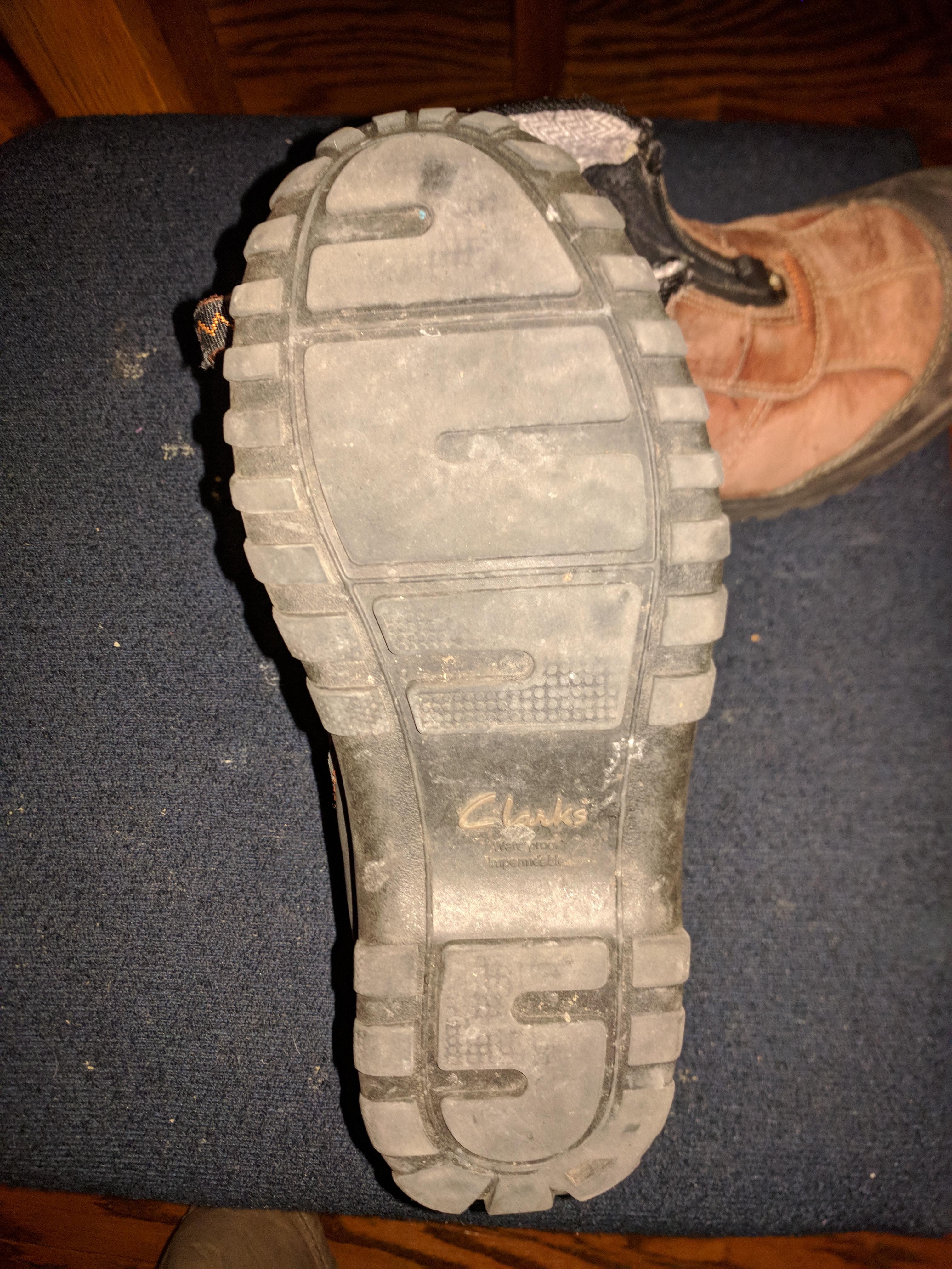
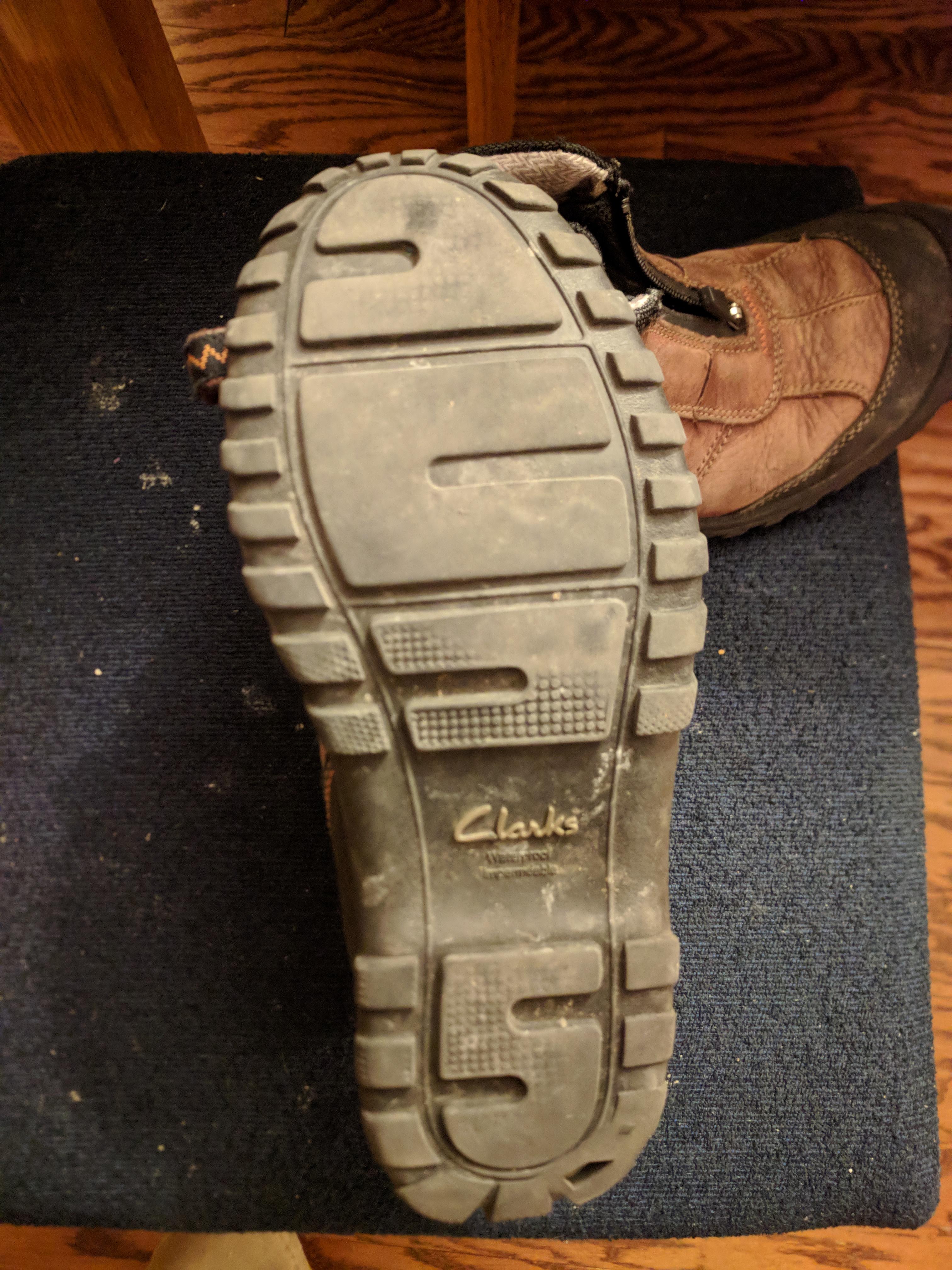
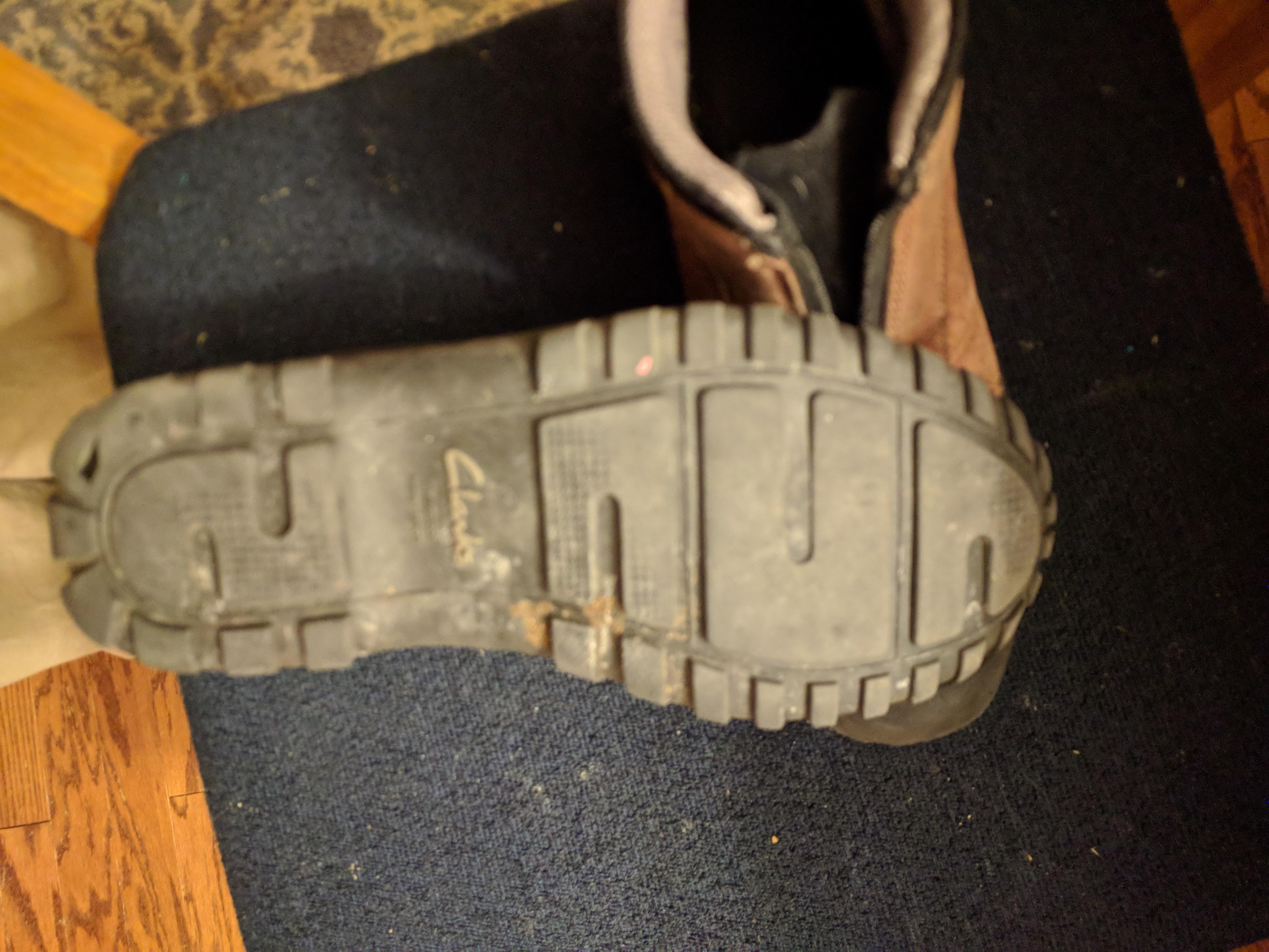
7.6 3d Shoe Recognition

Some background info: Shoe impressions are often left at crime scenes. In an ideal investigation, an impression left atthe scene of the crime is matched to the suspect’s shoe, placing them at the scene. However, it is not always that easy. An additional problem when dealing with shoes in the forensic discipline isshoes wear over time. When time elapses between the crime and recovery of the shoe, this processmay be more difficult: identifying marks may have worn away, or new marks may have been acquired due to additional wear. In order to understand the changes to an outsole of a shoe that may occur during the wear process, it is necessary to collect longitudinal data from across the shoe’s lifetime. These studies are needed to establish statistical models for shoe wear patterns and accumulated damage. In order to analyze data collected from these studies, it is imperative to develop a statistical pipeline to align and compare successive 3D scans over time. Manual alignment methods are time consuming, and do not scale effectively to large studies, because it is necessary to align hundreds of scans, observed at multiple time points, before any statistical analysis or modeling can be performed. To practically use longitudinal studies, the best approach is to develop statistical tools, to provide a pipeline in which to align and analyze two shoe scans.

The set up:

Ititally, the idea of the of the study was to use the data from the longitudial study in order to determine if one could predict wear, given pressure point matts and amount of steps and so on that was all part of the longitutidal data collection done previously. This idea has someone shifted. There is a large difference between the scans of the longitudial study that were conducted by hand scanning and those conducted using the turn table. The hand scan soles of the shoes have a wide variation not only on quality, but also on amount of shoe and direction of the scan. In order to simplify the inital processes and determining a pipeline for alignment, instead of the longitudinal shoe scans, the processes below are using a shoe that is scanned soly using the turn table to have some consistancy in the processing as we start to have a pipe line for at least alignment, then later using the longitudinal study add the extra information into the processing; amount of steps, weight,ect.

Steps: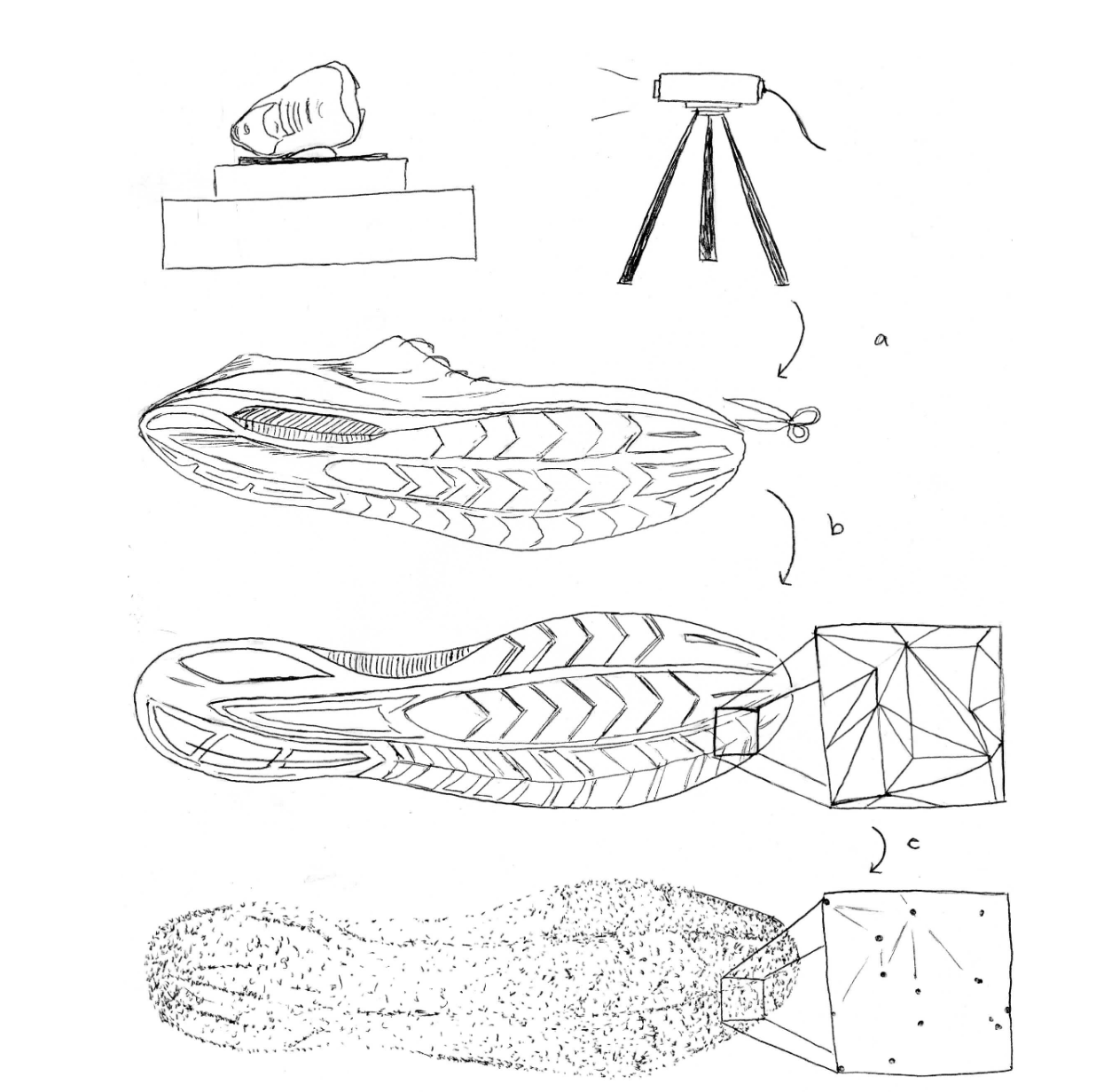

The shoe scans start as an stl file, however R does not work with stl files directly so they need to be transformed into a mesh object, in this specific case a triangle mesh object:

Mesh Objects: A triangle mesh object is made up of the following parts, sufaces, polygons, faces, edges and vertices.

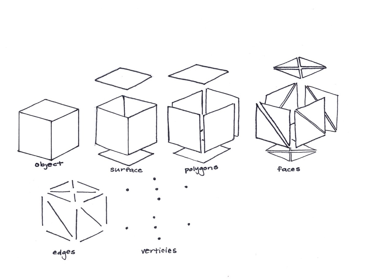
Looking at a mesh object at first:

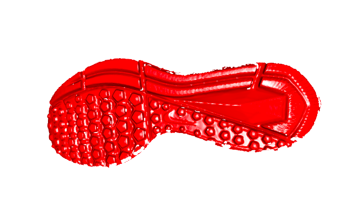
Some background: At first we wanted to try to simplify the mesh object to just the basic shape in order have simplicity when aligning. The idea of allignment is to take the most basic features, allign them, then by adding complexity of the soul, further allign the two different shoes. The idea is that we want to take a lower detail scan of shoe, allign it, then by adding complexity we can further allign the shoes. However the problem was realized that we are using a prediction to allign rather than the shoe, which ran into some quick problems. The next “attempt” at alignment came from a package called morph. In order to use this package, we needed to transform the data from a mesh object into a plane of points. In order to do this, we greated the function shoe_coord. This function takes a triangle mesh object, and looks at the vertices that make up each triangle. With a specific amount of vertices specified using the specification vert, shoe_coord, takes these vertices and maps them onto a x,y,z coordinate plane. Then using this coordinate plane, the allignment process began.

When working with coordinate systems, there was still not aligning, as each shoe was set on its own coordinate plane

Some attempts that have not really turned out well - Transforming the mesh objects to points aligned by the center of mass to overlay them detecting difference. 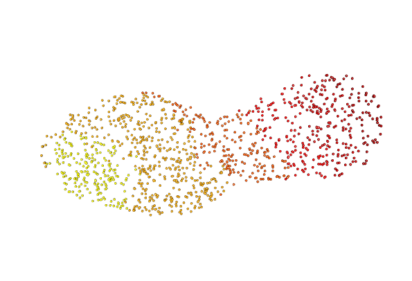- Problems - Isnt aligning properly as you can see

Principal Component Analysis: The basic idea of principal component analysis is to take a dataset with many variables, and simplify that dataset by turning the original variables into a smaller number of “Principal Components”. These principal components are the underlying structure in the data. Taking that data and giving a vector in directions where there is the most variance. Taking these egienvectors as the data, we can get a “flattened” version of our origianl shoe. This is done using singular decomposition: If the \(N \times p\) matrix X has rank r then it has a so-called singular value decomposition as \(X_{N \times p} = U_{N\times r} D_{r \times r} V'_{r\times p}\) where U has orthonormal columns spanning the column space of X, V has orthonormal columns spanning the colum space of X’ and D is a diaginal matrix of singular values. For ordinary principal components, the columns of V are called the principal component directions in \(\Re^3\) .

Once a shoe has been turned into coordinates from the verticies of a mesh object, we can use the function prcomp to get a transformation matrix.

Some notes on this:

• use vertices of 7 to decrease amount of points to match
• if you have too few points also doesnt work
• turn table works the best
• Sony are the best matches (the shoes I personally have scanned)

Point cloud alignment

• First looking at shoes with all vertices included:

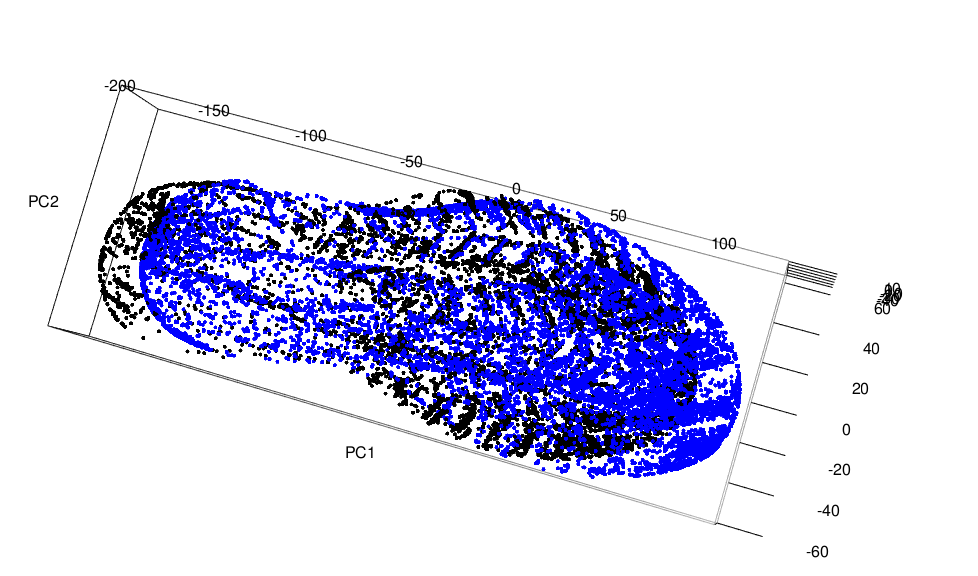
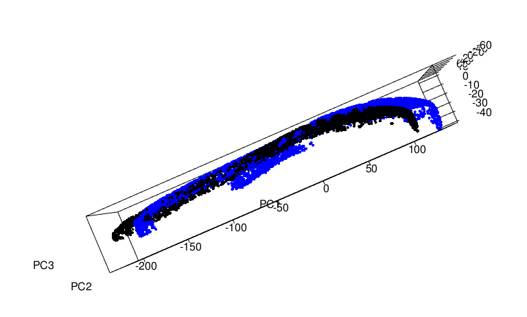
• Now the same shoe with fewer vertices included in the allignment

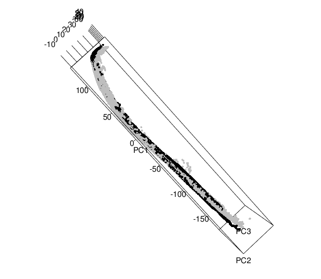
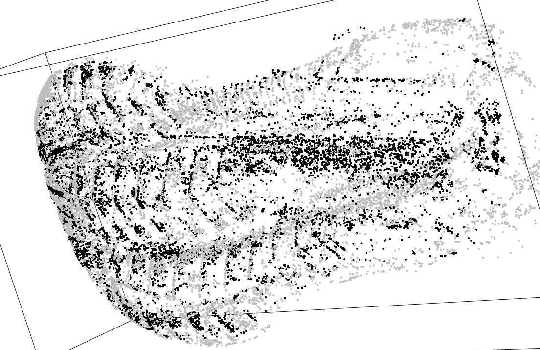
With these point clous alignments, the next step is to take the rotation matrix given by prcomp and apply it to the original mesh object since rather than comparing points that may or may not exsisit in comparison to each other shoes, as the vertices are not exactly the same on a mesh object from scan to scan of even the same shoe. prcomp gives a matrix that can be applied to a mesh object using a function called transform3d

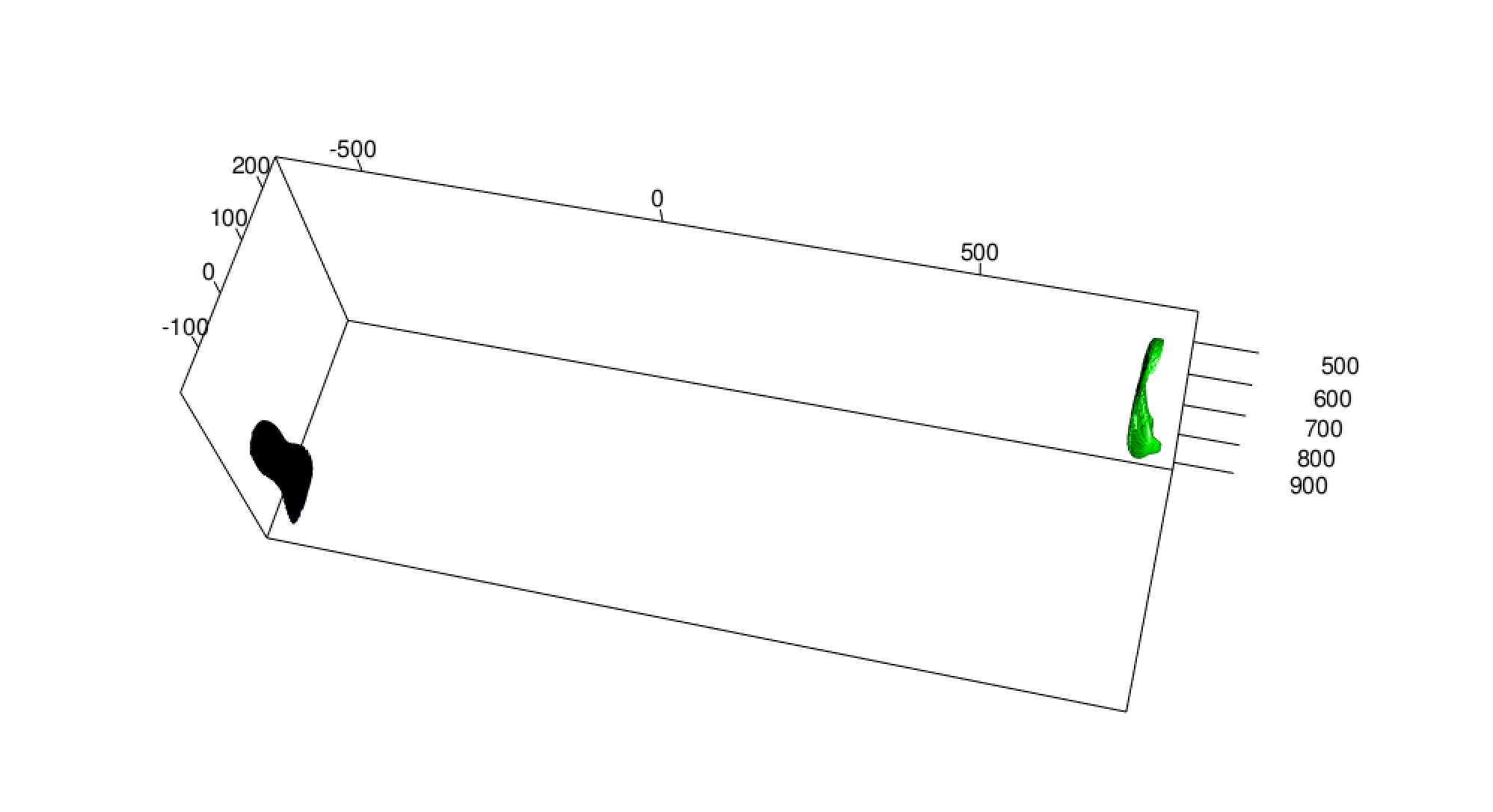
Once this was tried, it seems that the function prcomp isnt actually centering the data, although according to the code it should. So in order to overcome this issue when initially turning the stl file into a mesh object, a centering is performed using the barycenter of the shoe scan. In astronomy, the barycenter is the center of mass of two or more bodies that orbit one another and is the point about which the bodies orbit, since we are obviously only dealing with one object, the barycenter can be thought of as the center of mass for the shoe scan (the center of mass of a distribution of mass in space is the unique point where the weighted relative position of the distributed mass sums to zero). This puts the point (0,0,0) in the center of the shoe rather than the center being close to the 300s as before

Centering

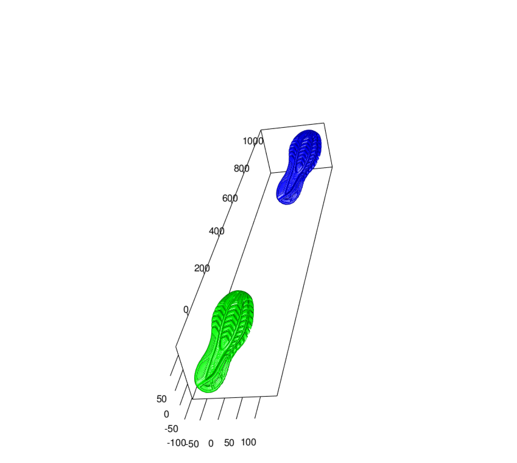
The blue shoe is the original shoe grab, where the green shoe is now the shoe that has been centered on the center of mass. Now we can start with two shoes that at least have the same “center” point before principal component analysis is completed:

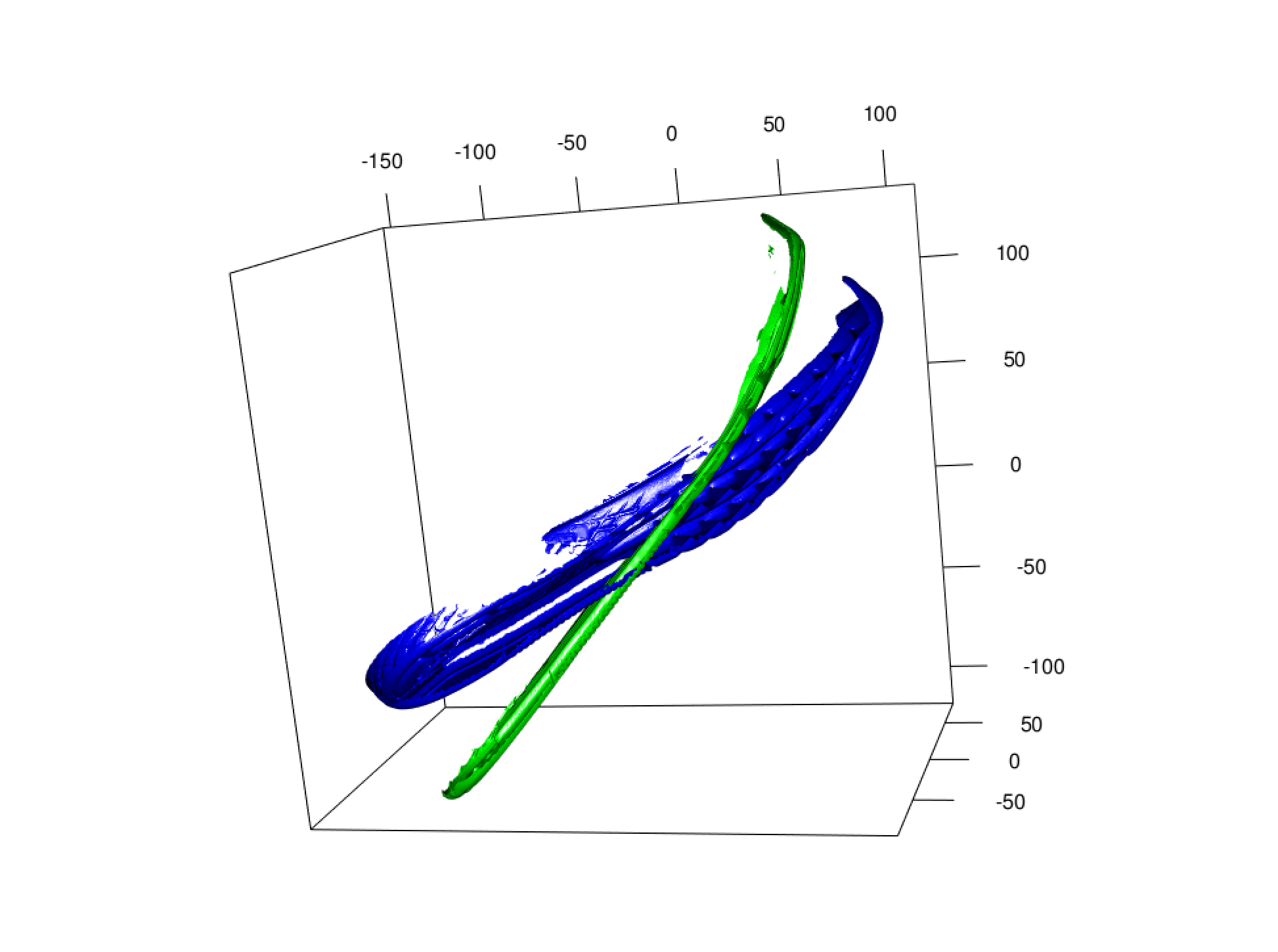
Once the shoes themselves have been centered, then PCA can be compleated on the shoes themselves:

PCA after centering

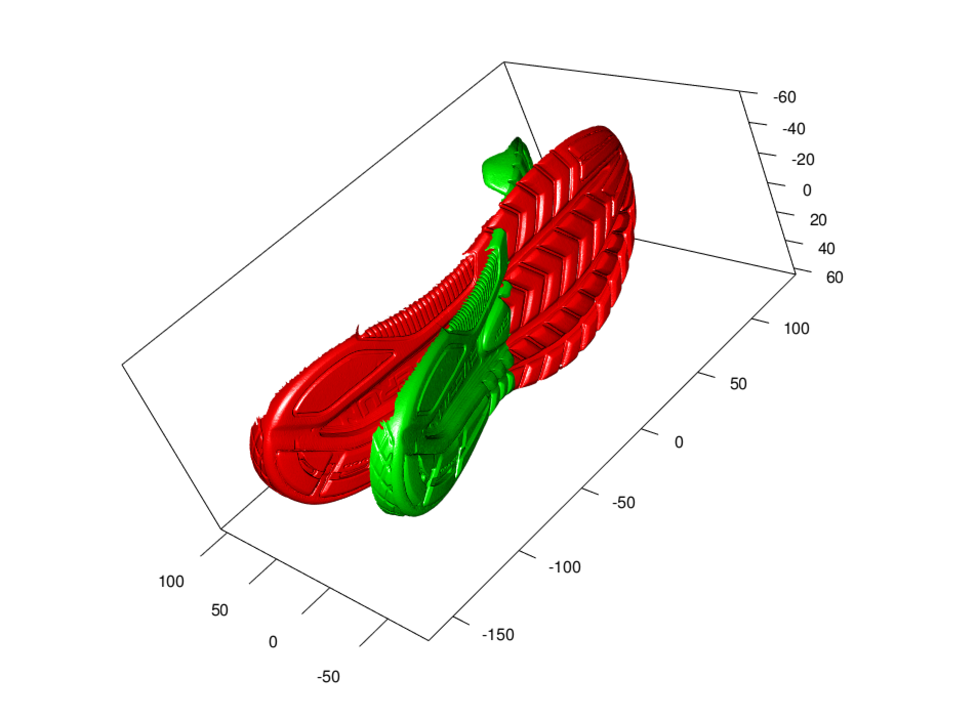
The Green shoe is the original shoe grab centered, where the red shoe is now after PCA has been applied. Then using the PCA for both of the two scans we can get the following map of the two shoes with their given principal component rotation matrix applied:

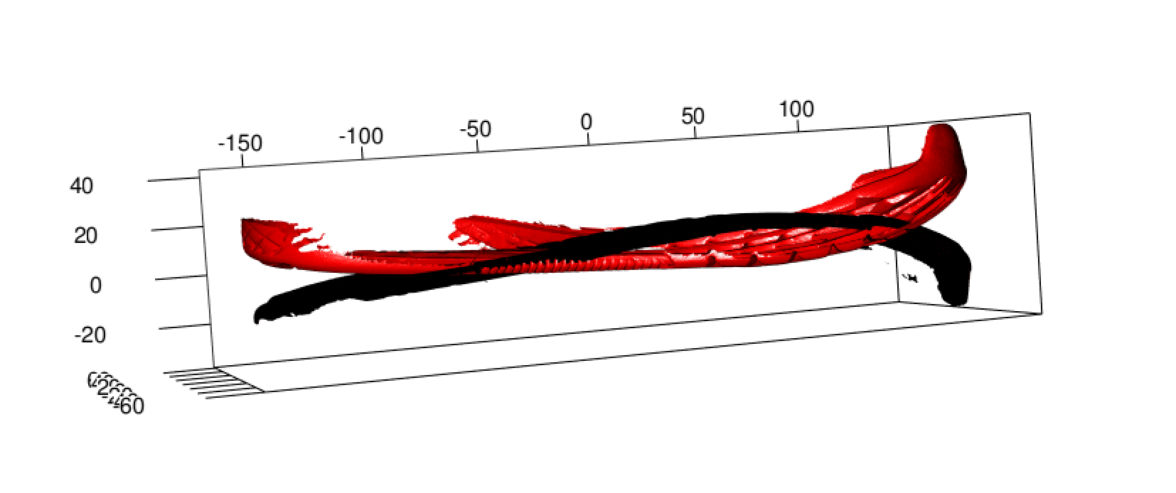
As you can see although they are on the same plane, they are not exactly allign. In order to get them aligned a matrix of 1s and -1 needs to be applied in some order, minimizing the RMSE

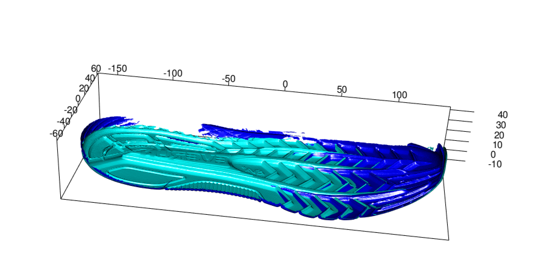
Once the PCA has done the initial alignment, then a secondary alignment needs to be done using Itterative Closest Point, to do this a landmark must be established. One cant just use the PCA, the way that the initial scans are only of the soles, which change as they wear, so we are trying to allign something that is not there anymore. The idea landmark will give a spot in the shoe that will not change, the arch or a large indent, in order to find a proposed landmark, we are attempting to use the maximum distance in z.

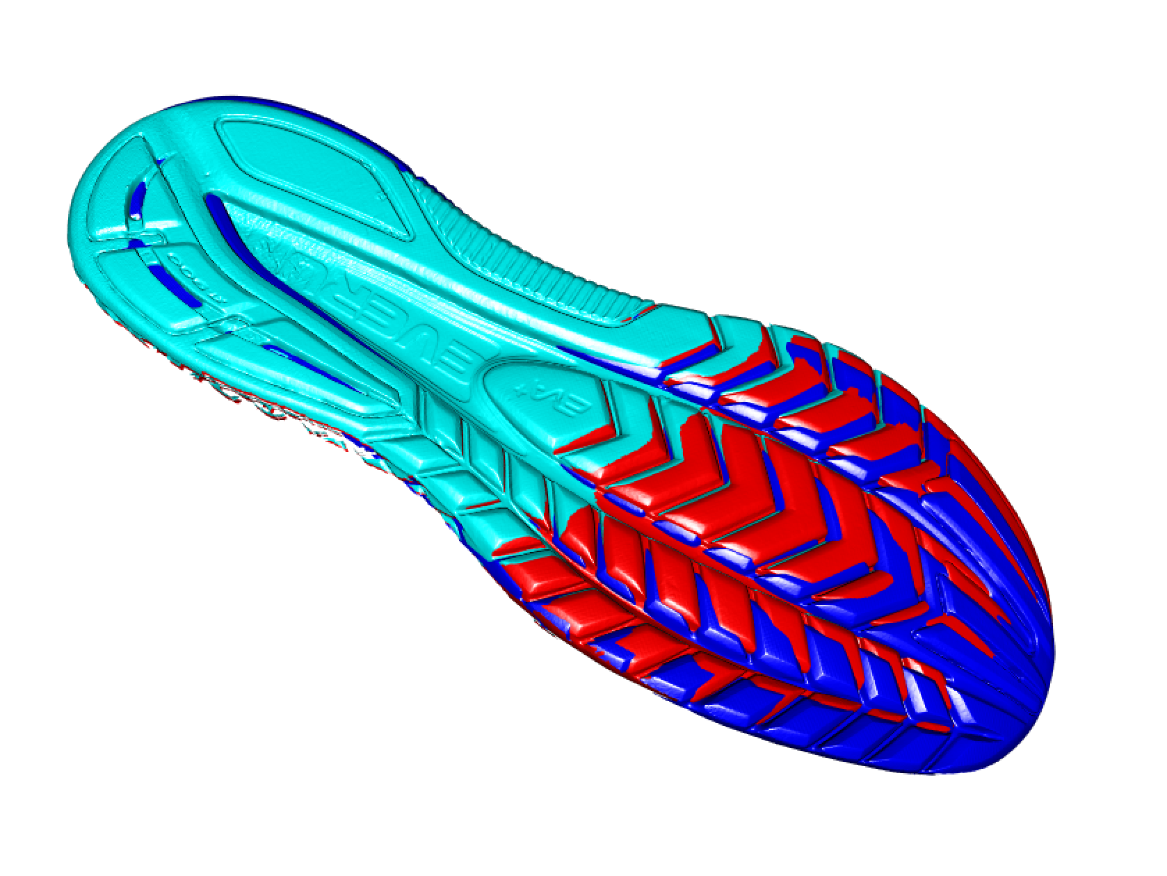
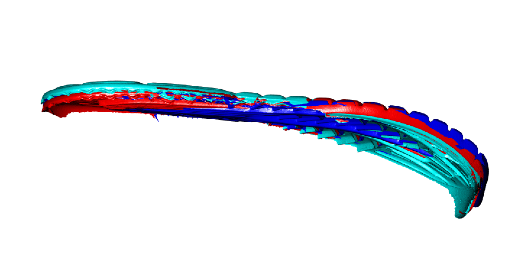
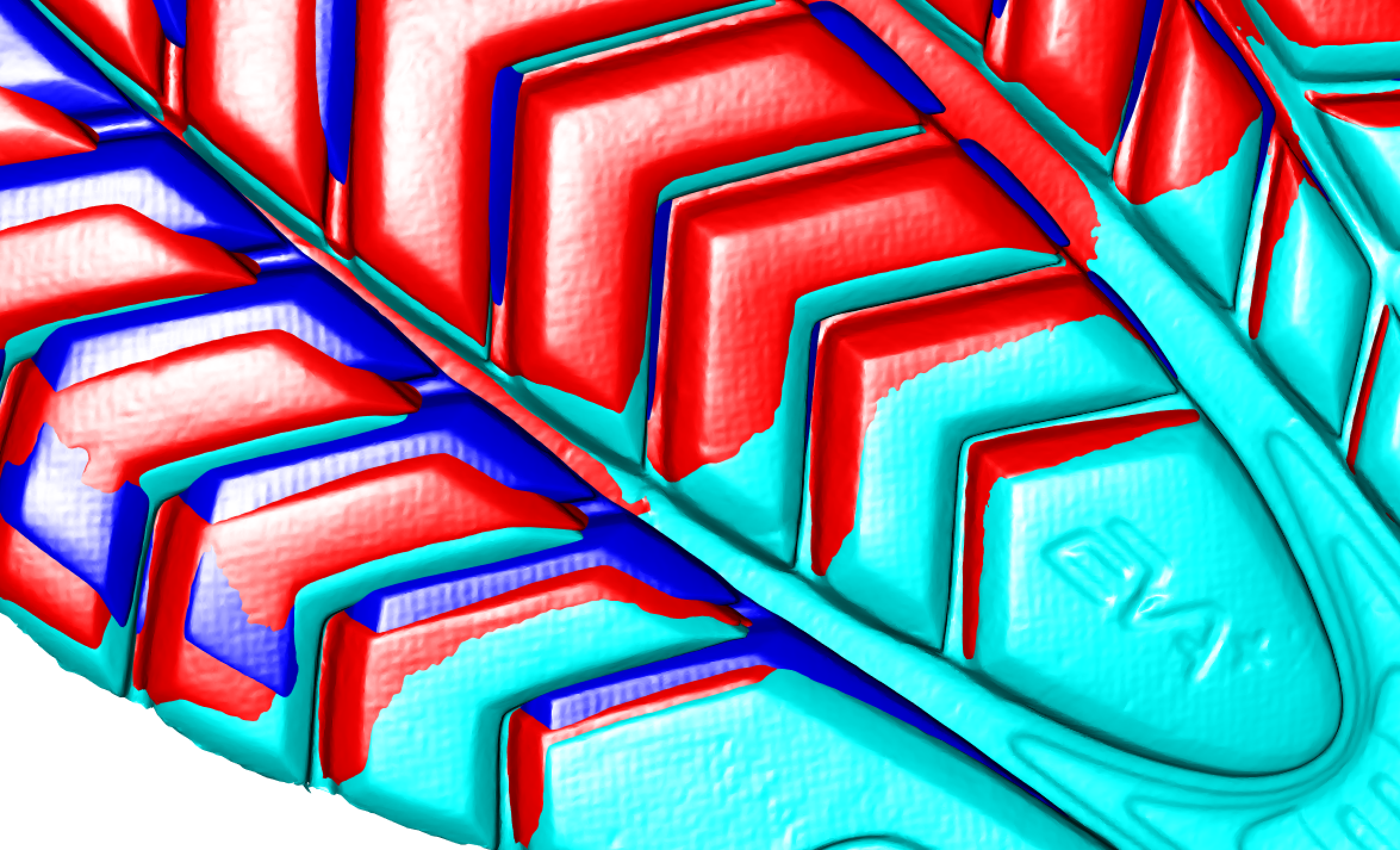
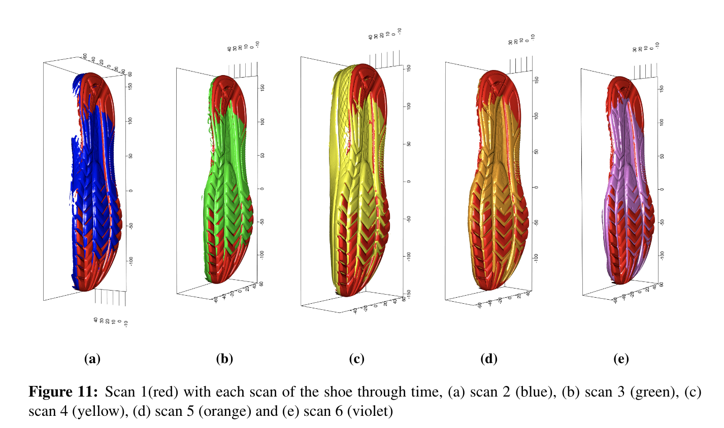
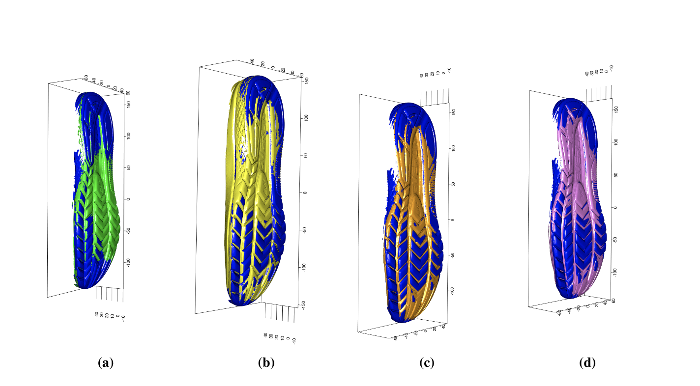
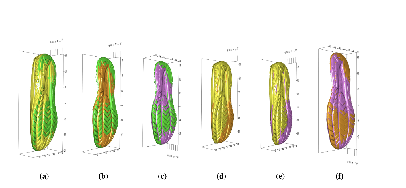
Automated Alignment:

In order to align the shoes through an automatized process, we need to use the following steps.

1. We begin with the two mesh objects of the same shoe at different time points, say time i and time j.Then using the barycenter, or center of mass, we center the shoes on the same x,y,z, coordinate system.

2. After the shoes are then centered, they are transformed into a point cloud made up of the verities of the triangle mesh object.

3. Using these two coordinate systems. Principal component analysis is performed. This gives us a 3X3 rotation matrix in which to transform the original mesh object by the PCA rotation matrix.

	PC1	PC2	PC3
x	0.5603136	-0.2618793	0.78579127
y	0.3038740	0.9475434	0.09910676
z	0.7705253	-0.1832507	-0.61049973

4. Due to the nature of PCA, the rotation matrix that we are using is not unique. Further more it often times has a negative determinate. If this happens, we need to rotate the mesh shoe object by a matrix whose diaginal is (1,1,-1). Leaving us with a positive determinate.

5. After this is done, there is no guarantee that the two shoes although sharing the same space in x,y,z where x is the length of the shoe, y the width and z the depth, will be in the same direction.

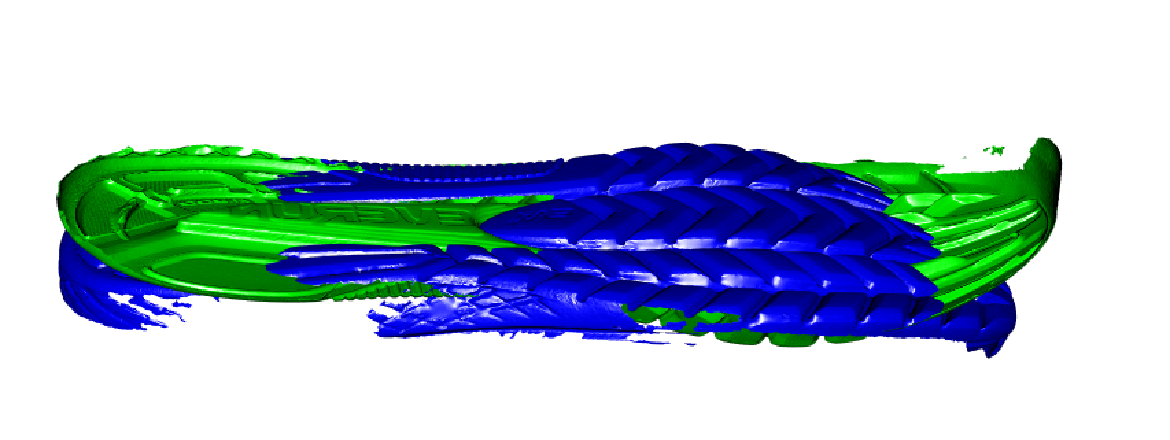
In order to correct for this we need to rotate the shoes by 180 degrees in x,y,z or a combination of those directions. There are 8 possibilities of those rotations:

1. rotation around the x-axis 180 degrees
2. rotation around the y-axis 180 degrees
3. rotation around the z-axis 180 degrees
4. rotation around the x-axis 180 degrees and the y-axis 180 degrees
5. rotation around the x-axis 180 degrees and the z-axis 180 degrees
6. rotation around the y-axis 180 degrees and the z-axis 180 degrees
7. rotation around the x-axis 180 degrees and the y-axis 180 degrees and the z-axis 180 degrees
8. No rotation is needed

there are only 4 unique matrices to deal with

Matrix Rotations

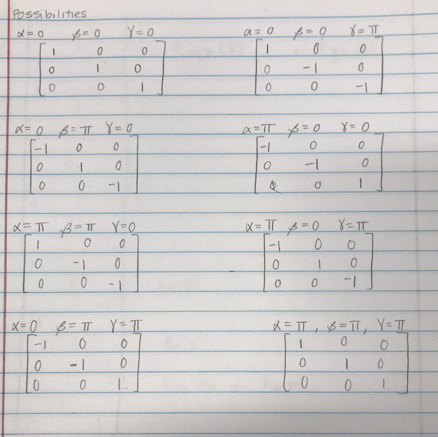
In order to choose which one of these matrices, the first shoe scan in time is set as the base scan. Then each of the four matrices described above is applied to second scan. After each rotation, the distance between the first and second scan is measured. The matrix with the smallest distance is used as the rotation matrix, and is applied to the second shoe. For example, with scan 1 and scan 2, the four matrices lead to the following 4 distances: 2.153458, 9.124214, 9.117095, and 6.234845. Thus scan 2 is rotated by the matrix of the diag(1,1,1).

6. Once the shoes are initially alligned, ICP is applied with an iteration of the aligners choosing. Once ICP has been performed, the distance is again measured and recorded.

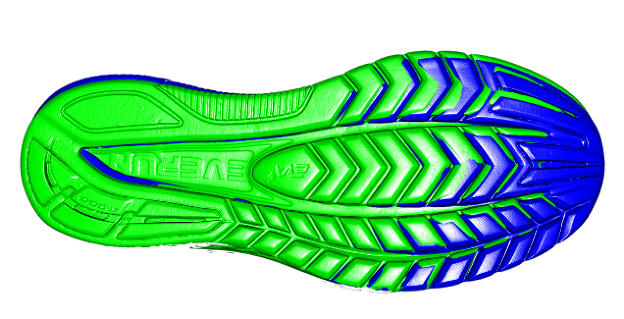
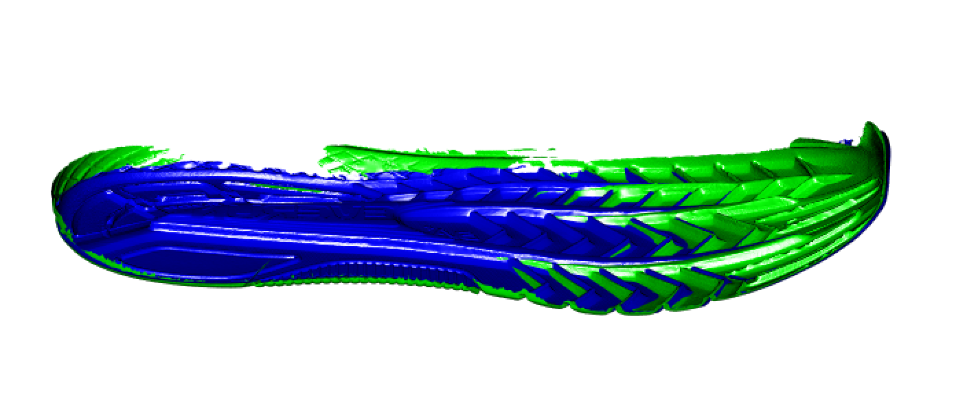
Here the final distance is 0.9791678 cm

How distance is being measured: In this process, we set the first scan as a base scan (here scan 1). This scan does not move through the process. Once this scan is set, using a K-D tree method the shoe is divided up into sections until there is only one vertex in each section. This process is done to the second shoe as well.

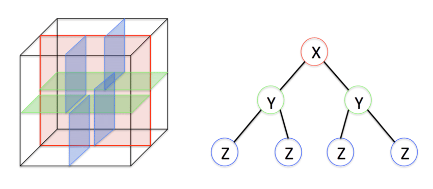
K-D construction is as follows divide the points in half by a line perpendicular to one of the axes, in each tree. Then recursively construct k-d trees for the two sets of points, the two points corresponding to the verities of the triangles. Think of it as this, we first choose a shoe to be set. In this case shoe scan 1. Then for each one of the verticies of a triangle we draw a ball with radius then we start epsilon to be 0 and expand it till you hit the closest section with a specified point.

Each point is then pair with the closest euclidean distance corresponding point.For two vectors or two vectors (x_1,y_1,z_1) and (x_2,y_2,z_2), the euclidean distance is found by: \[ \sqrt(\sum^n_{i=1}(q_i-p_i)^2) \]

This is repeated for the set iterations, or until epsilon is deemed small enough. Each time the distance is measured, but the K-D tree sectioning remains the same through the process. This gives us N distances for the number of iterations. We return the final N iteration’s distances from each set of verities. The mean of these distances is then computed, giving us a distance metric. This is used to find the magnitude of the distance between the two shoes. This distance is consistent for each processing of two shoes (i.e. if you run scan 1 and scan 2 through this process, you will still get the same distance of 0.98. However, if you switch the positions of the shoe, making scan 2 the base you will get a different result, 2.243478)

Understanding the distance:

Once we have the distance, we want to understand where the wear is occurring, plotting the distance on the base scan of scan 1, we see the distance to scan 2 looks like the following:

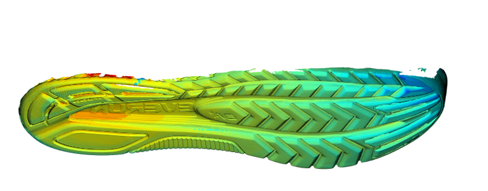
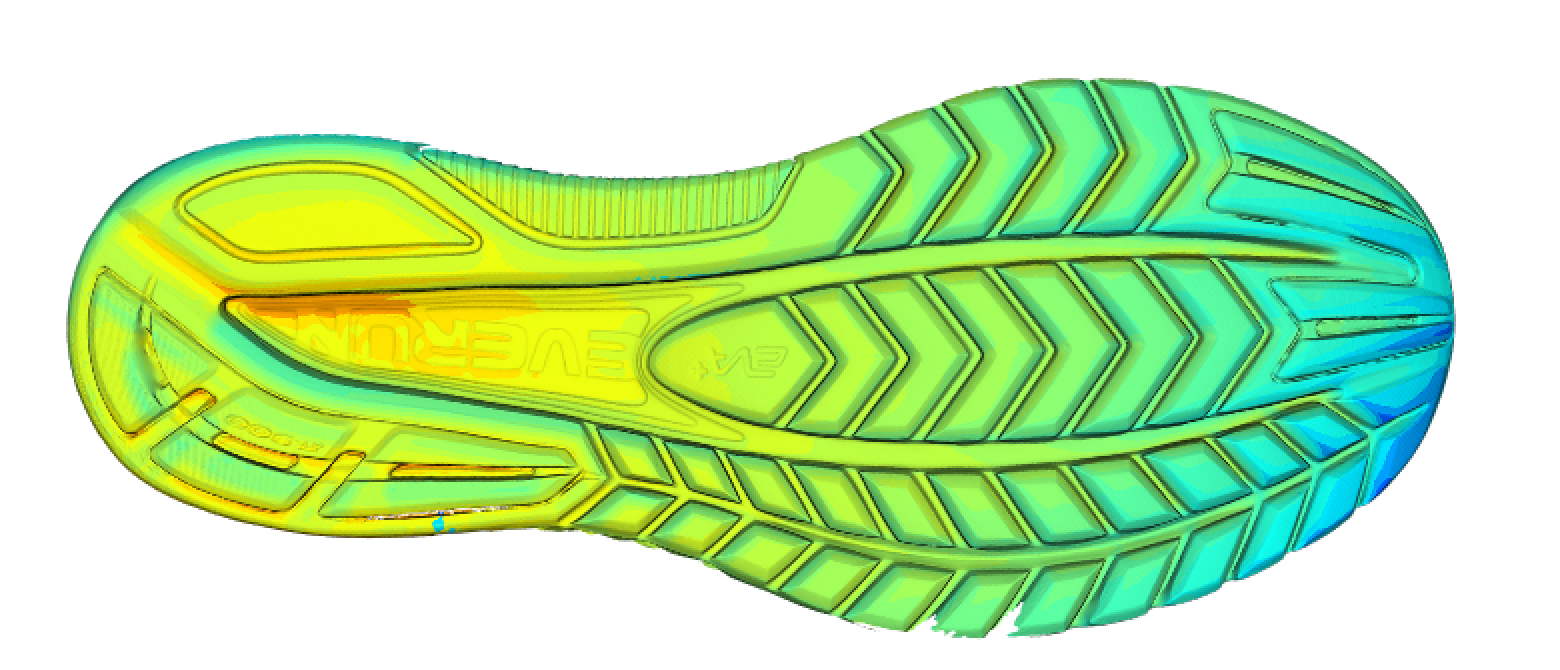
Some Issues through the process:

1. Inconsistency of scans: As we have seen the cropping of the scan is inconsistent, i.e. where the scans were cut

2. How ICP is being measured: It is unclear how much ICP is changing after each iteration. For example, in our scan1 vs scan 2 shoes if we take the mean distance after 1 iteration, then 2, up to 20 iterations we get the same mean. (next step is to go further out to see if it changes, or look at the distribution of distances after each iteration and not just the mean, to see if the tails are changing.)

7.7 Shoe outsole matching using image descriptors

7.7.1 Method 1: Edge detection and MC (MC-COMP)

Under the revision by Journal of Applied Statistics,

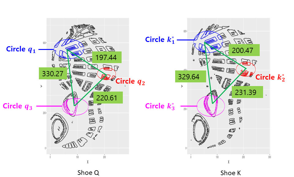
Comments by reviewers

Compare your predictive accuracies on the number of circles (more or less than 3).

In the previous matching, we found three circular regions in red. As reviewer requests, we selected the additional three more circles in blue. We tried the same set of mated and non-mated matching in training and testing set.

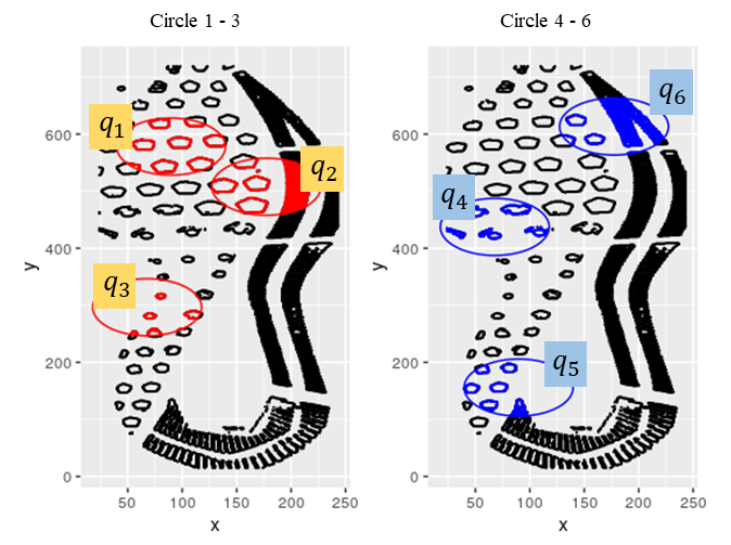
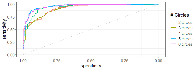
We get the average of the similarity values by the number of circles. The random forest is trained on the set of results summarised by the number of circles.

When there are five and six circles found in the questioned shoe, then the AUC is the largest as 0.96 in the test set.

7.7.2 Method 2: SURF detection and MC on degraded impressions

Accepted by Statistical Analysis and Data Mining in Feb. 2020.

Comments by reviewers

1. Generalization (Fingerprints, Photos of faces, … )
2. Other classifiers, besides the random forest.
3. Variable importance

7.7.3 Research 1: Features

Previously, features such as edge, corner, SURF were extracted to match shoeprints. The goal of this project is to find other image descriptors as image features for shoe print matching.

Image descriptors

• SURF(Speeded Up Robust Features)- blobs
• KAZE - blobs
• ORB(Oriented FAST and Rotated BRIEF)- corners

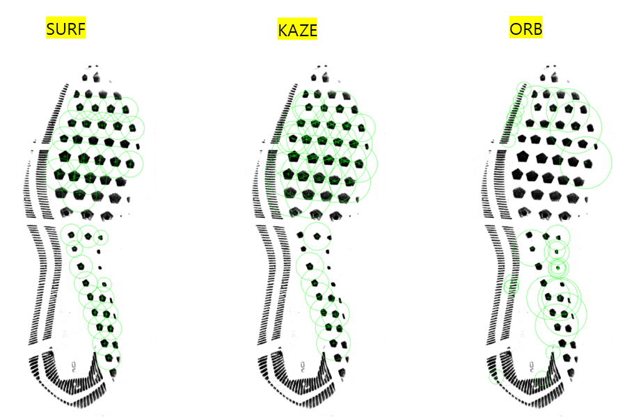
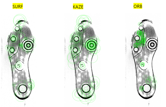
Image matching

• CSAFE data - Nike size of 10.5 and Adidas size of 10 will be used to construct mated and non-mated matching
• Features will be combination of strong 100 points of KAZE, ORB, SURF.

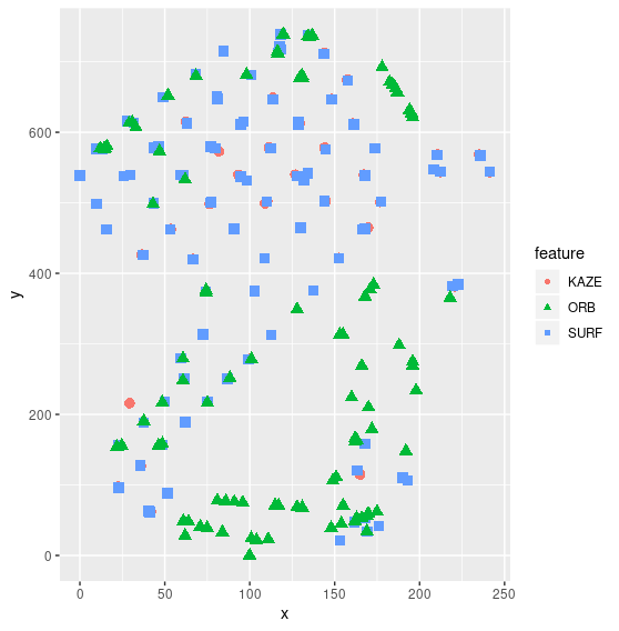
7.7.4 Matching on clean and full images with several features

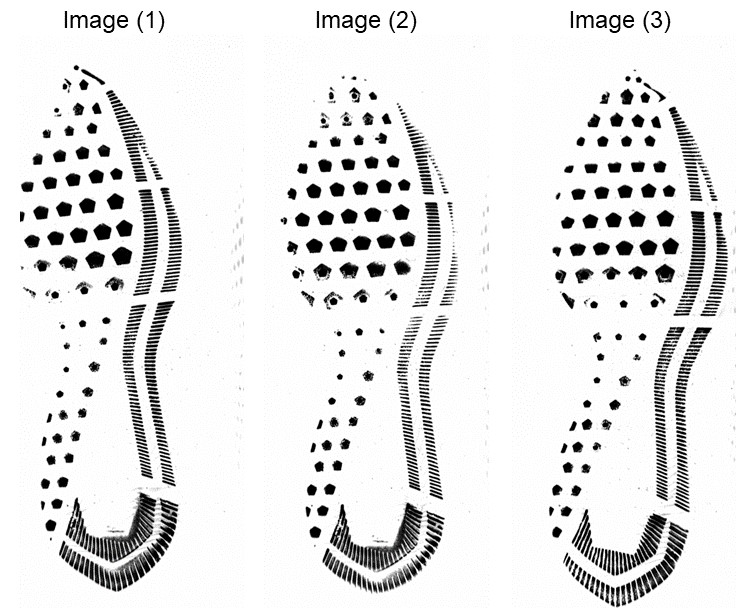
• Mates : Image (1) and (2)
• Non-mates : Image (1) and (3), Image (2) and (3)

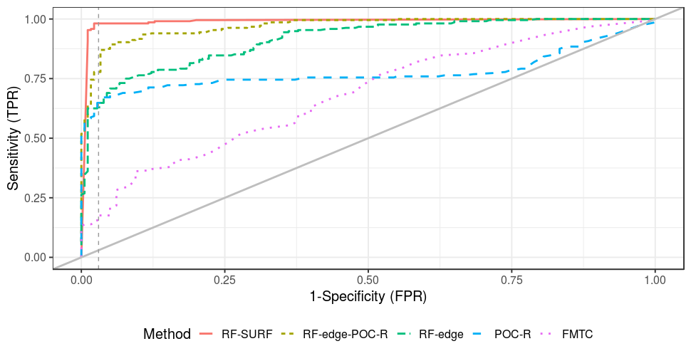
Performance evaluation using

• SURF 500
• KAZE 500
• ORB 500
• SURF 100 + KAZE 100 + ORB 100
• SURF 200 + KAZE 200 + ORB 200
• POC (Phase-only correlation)
• FMTC (Fourier Mellon transformation correlation)

Example graphs of mates:

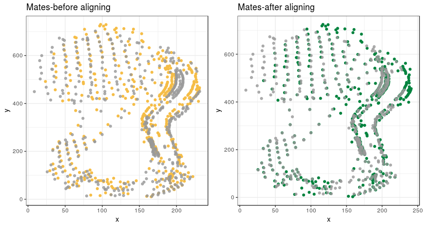
Example graphs of non-mates:

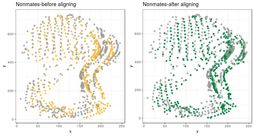
Example matching table using SURF 500:

Class	Clique size	Rotation angle	% Overlap	Median distance of OP
Mates	18	2.11	0.5646	0.78
Non-mates	9	6.43	0.1208	1.39

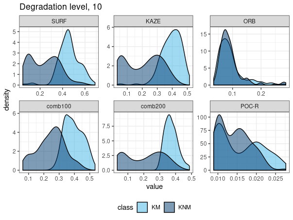
Density plots:

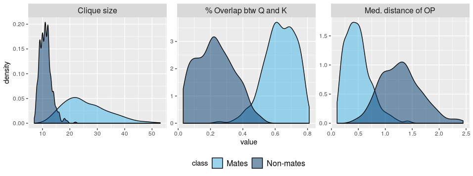
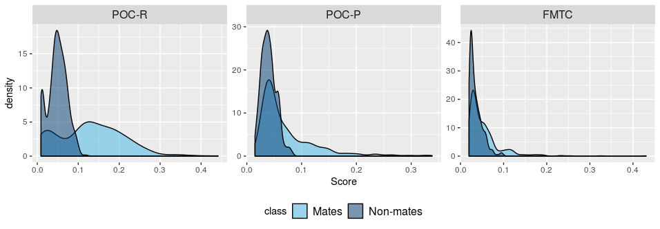
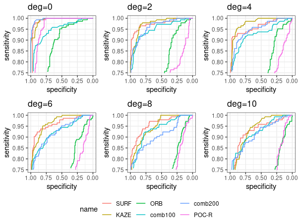
ROC curves on test comparisons:

7.7.5 Matching on degraded and partial images

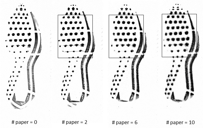
Example of degraded images:

Example crime-scene like images on dust from the data by Speir’s group: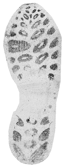

Density of mates and non-mates by features:

ROC curves by features:

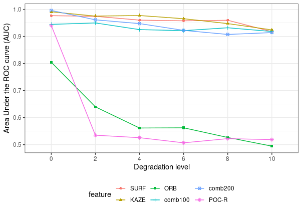
AUC values by features:

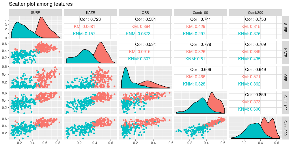
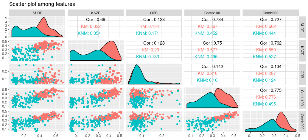
Relationship among similarities (% Overlap) by feature-types

• Overlap feature (% overlap after the alignment) in the degradation level, 0

• Overlap feature (% overlap after the alignment) in the degradation level, 10

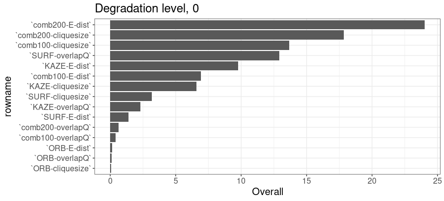
Random forest training for the variable importance

• Trained the RF, in the degradatino level of 0 and 10, on the class with the variables of all similarities by each feature type.

• Degradation level 0

• Degradation level 10

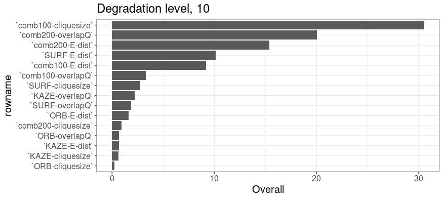
7.7.6 Research 2: Impact of weight to outsole scans from EverOS 2D scanner

Analysis setup:

• Shoes: 5 pairs of Nike Winflow 4, size 10.5 (Brand-new shoes)
• Participants: Person 1 (weight aa lb)and person 2 (bb lb)
• Weights: 2 weight vests (20 lbs and 12 lbs)
• Weight variations: W1(P1), W2(P1 with one vest), W3(P1 with two vests), W4(P2), W5(P2 with one vest), W6(P2 with two vests)
• W1 \(=\) 155.2 lb, W2 \(=\) 173.8 lb, W3 \(=\) 187.6 lb, W4 \(=\) 178 lb, W5 \(=\) 197.4 lb, W6 \(=\) 211 lb

Result1:

• Shoe is fixed to left side of shoe1.

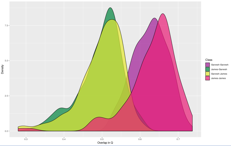
Result2:

• Purple, green: comparison between repeated replicates from the same shoe, W2-W2, W4-W4.
• Comparison between weights W2 and W4: weights are almost the same.
• Yellow: comparison when shoe is fixed to shoe1-L.
• Red: comparison between shoe1 – shoe2-5.
• Shoes are never used.

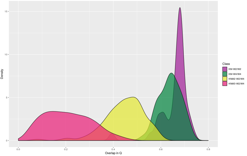
Discrimination among groups

Let’s simplify the question; Is the person effect significant?

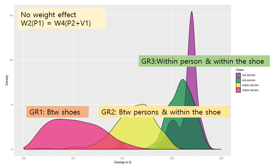
• Initial analysis
  • Cluster analysis; hcluter
  • Principal component analysis (PCA)
• Are groups significantly different?
  • Multivariate Analysis of Variance (MANOVA)
  • Multi-Response Permutation Procedurs(MRPP)
  • Analysis of Group Similarities (ANOSIM)
• How do groups differ?
  • Discriminant Analysis (DA)
  • Classification and Regression Trees (CART)
  • Logistic Regression (LR)

7.7.7 Research 3: MC + CNN

Idea:

1. Align two images using MC.
2. Calculate similarity features.
3. Ask CNN to learn similarity features.
4. Combine 3 and 4. Use ResNet-50 to get a final similarity value.

### Additional features from descriptors

Much of the outsole matching already done at CSAFE is based primarily on the geometric locations of SURF features. While this is apparently useful, the utility of SURF and other computer vision features (such as BRISK, ORB, and KAZE) can go far beyond location. Most of the work done has also been on images produced using the EverOS 2D scanner. Location features from these images are relatively easy to align, but with different image types -such as those made using fingerprint powder- alignment becomes much more difficult.

When a SURF (or other feature type) is detected in an image, several features are extracted. Each SURF is a detected “blob” from an image. Features from a SURF include Sign of Laplacian, orientation, location, metric, and a 1x64 vector of descriptors. Essentially these several features describe characteristics of the blob like color intensity, change in intensity, change in pattern, blob direction, etc.

Between two different images if two SURFs have a matching sign of Laplacian, the distance between the two 1x64 descriptor vectors is measured. If the distance is below a specified threshold the two SURFs are considered matching.

Sign of Laplacian

64 descriptors

When SURFs are matched, a matrix is returned with indices of matching SURFs and the measured distance. Matched features are illustrated here.

Clearly many of these “matched” SURFs -based on metric- are not actually corresponding parts between images. To make more precise which SURFs match, I use the maximum clique from the shoeprintr packages to align the SURF points based on location. Once aligned, Euclidean distance is used to find the closest point(s) in image 2 to each point in image 1. Now there are two sets of matching indices. The index pairs which overlap between the two sets are considered certain matches.

The number of “certain” matching SURFs and the metric between SURF descriptors can be used as two additional features for image pair comparison.

Useable features

• Clique Size
• Rotation Angle
• % Overlap
• Median distance of OP
• Certain SURF matches
• Max SURF match corr

We’ve trained 2 different random forests using these features from image pairs.

The first random forest uses 115 pairs of images using matching soles with the same stepping style and 116 pair of images of the same shoes with different stepping style. The random forest classification accuracy using leave one out cross validation is 92%

Different step type average variable values

Class	Clique size	Rotation angle	% Overlap	Median distance of OP	Certain SURF matches	Max SURF match corr
Same steps	8	3.97	0.1992	1.21	13	0.9523
Dif steps	6	14.04	0.0169	0.99	0.487	0.2236

RF Variable importance

Variable	Importance Score
Certain SURF matches	100.000
% Overlap	14.951
Max SURF match corr	14.059
Rotation angle	4.484
Median distance of OP	2.359
Clique size	0.000

The second rf is trained from 115 images of matching shoes with the same stepping style and 116 images of non-matching shoes with the same stepping style. The random forest classification accuracy was also 92%

Match v. non-match average variable values

Class	Clique size	Rotation angle	% Overlap	Median distance of OP	Certain SURF matches	Max SURF match corr
Mates	8	3.97	0.1992	1.21	13	0.9523
Non-mates	6	9.26	0.0164	1.24	0.836	0.2821

RF Variable importance

Variable	Importance Score
% Overlap	100.000
Certain SURF matches	34.044
Max SURF match corr	26.937
Rotation angle	2.221
Median distance of OP	2.213
Clique size	0.000

Improvements to be made

When two images using fingerprint powder are are from the same shoe and with the same stepping style, the alignment using maximum clique is generally good. However, when the sole images are not mates the alignment is occasionally not good. The alignment is especially poor when the step style changes.

So far, other existing methods haven’t shown any more effectiveness in aligning shoes than the maximum clique. It would be useful if features could be made from the SURF descriptors which could be used to compare shoes without needing to align the images.

7.8 Matching shoe prints with ccf

7.8.0.1 Steps to match two shoe scans

## Error in library(tidyverse): there is no package called 'tidyverse'

1. Training/Test sets

• Training set: Shoe scans from 10 shoes that have size 7 and were scanned twice at visit1. Then, 10 matching pairs and 90 non-matching pairs are made. e.g., a matching pair is scan1 and scan2 from the same shoes; a non-matching pair is scan1 from one shoe and scan1 from another shoe.

• Test set: Shoe scans from 10 shoes that have size 7.5 and were scanned twice at visit1. Then, 10 matching pairs and 90 non-matching pairs are made.

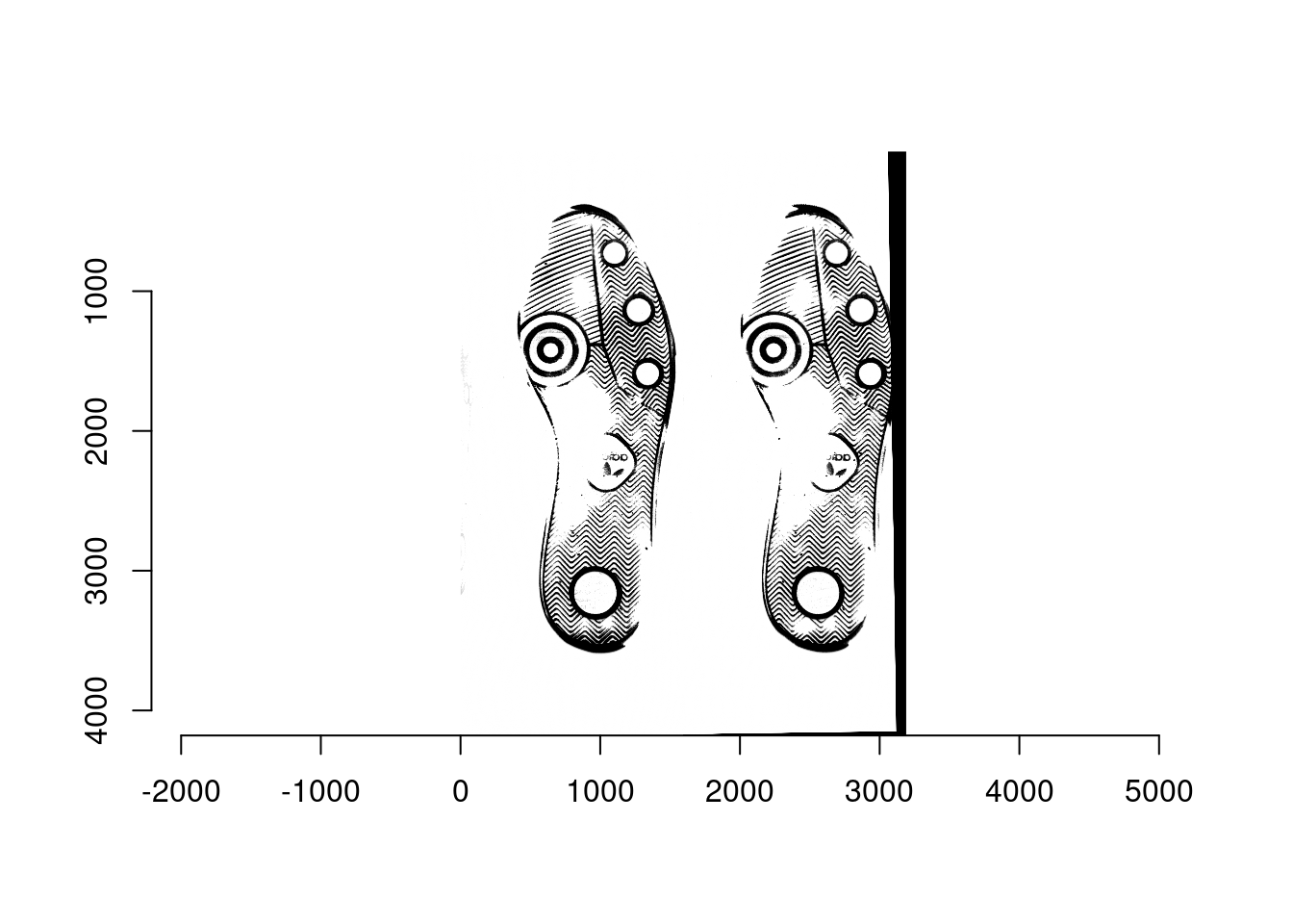
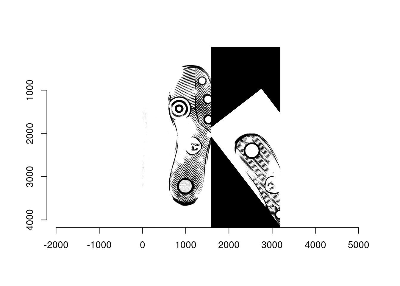
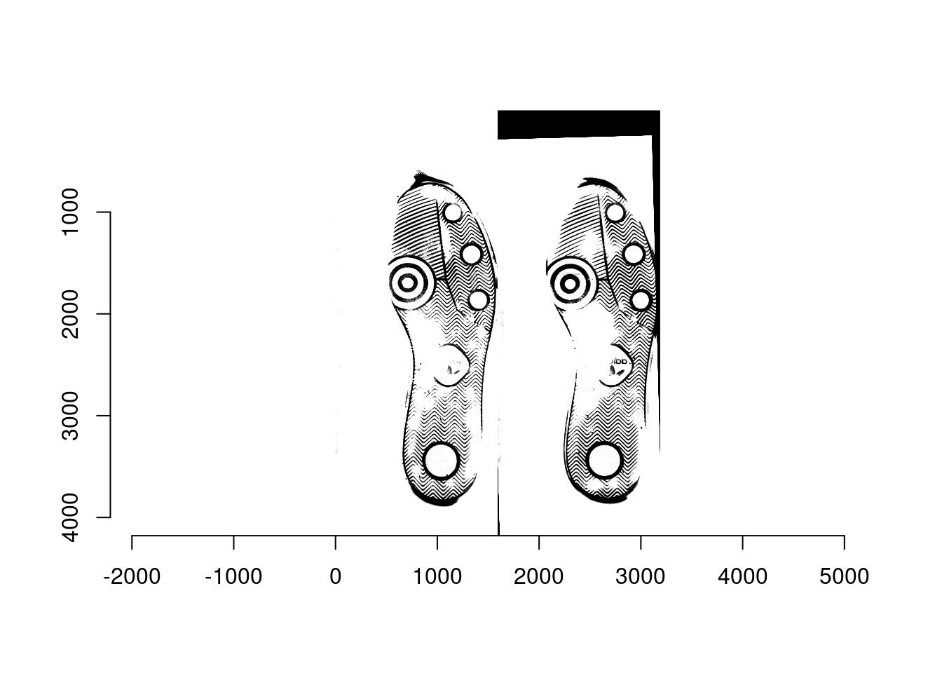
2. Align each matching/non-matching pair in training and test sets using Matlab. For each pair, one is reference image and the other is moving image to be aligned with the reference image. For example,

• Ex1: A matching pair: scan1 (left; reference) and scan2 (right; moving) from shoe1

• Ex2: A non-matching pair: scan1 (left; reference) from shoe2 and scan1 (right; moving) from shoe1

• Ex3: A non-matching pair: scan1 (left; reference) from shoe3 and scan1 (right; moving) from shoe1

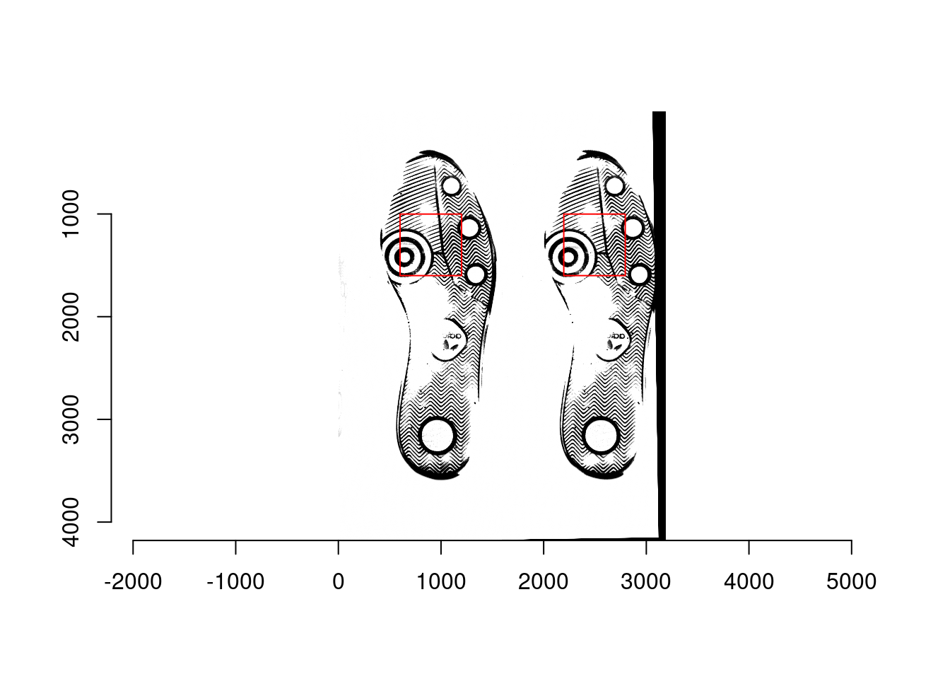
3. Determine 600px by 600px square coordinate for all of the reference images; the location of square is the same for each reference image. For example, the bottom left corner is at (601, 1001) and the top right corner is at (1200, 1600).

• Ex1: A matching pair: scan1 (left; reference) and scan2 (right; moving) from shoe1

• Ex2: A non-matching pair: scan1 (left; reference) from shoe2 and scan1 (right; moving) from shoe1

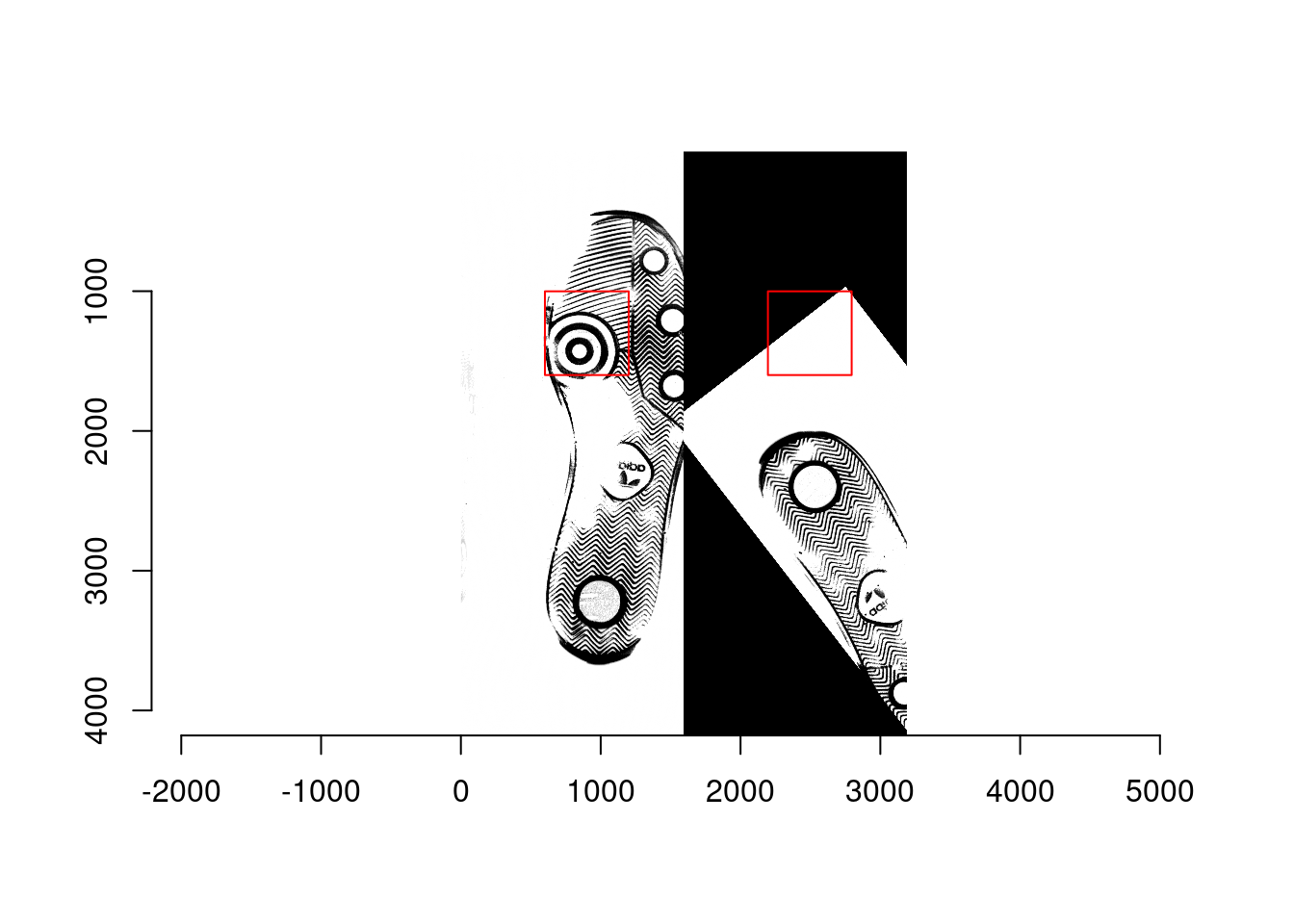
• Ex3: A non-matching pair: scan1 (left; reference) from shoe3 and scan1 (right; moving) from shoe1

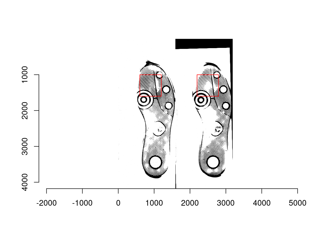
4. Extract the 600px by 600px square from both reference and moving images in each matching/non-matching pair, and then split each square into 36 smaller squares that are 100px by 100px. As a result, there are 36 100px by 100px squares are obtained from the reference and moving images, respectively, in each pair.

• Ex1:

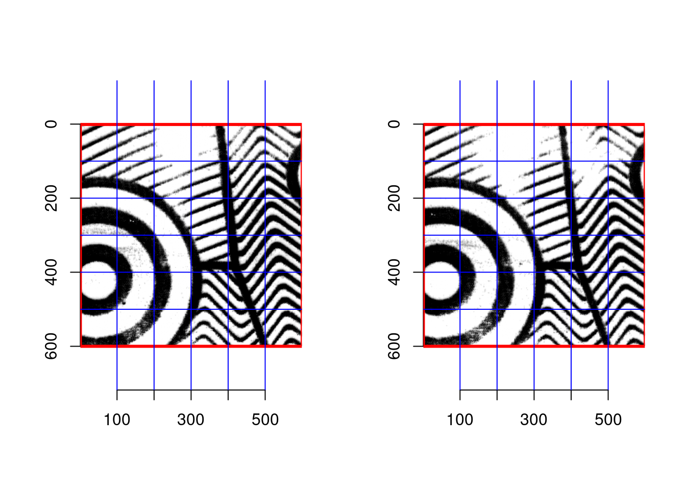
• Ex2:

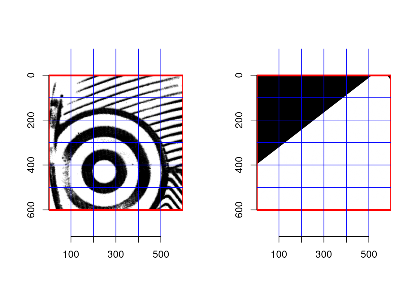
• Ex3:

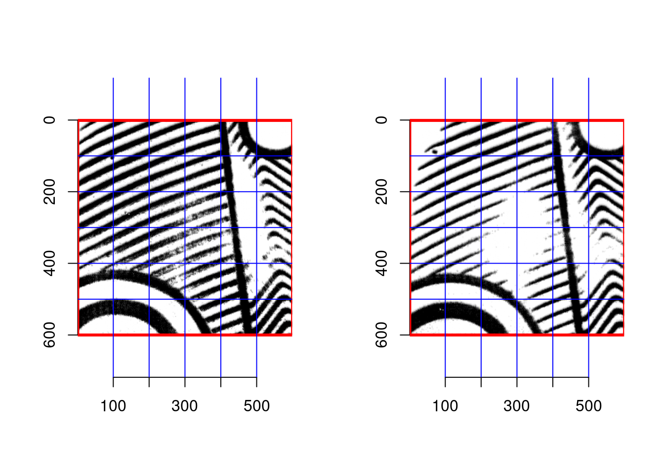
5. Compute maximum cross correlation function from a small square of a reference image and its corresponding small square of the moving image. Consequently, there are 36 maximum ccf and their (dx, dy) obtained from each matching/nonmatching pair. Summarize ccf, dx, and dy so that only a single set of features from them is made from each pair.

##   fft_ccf_mean fft_ccf_sd fft_ccf_range      x_mean       x_sd x_range
## 1    0.9828075 0.01881824     0.1086021  -1.0277778  0.1666667       1
## 2    0.6441020 0.31670677     0.9436405 -14.7500000 21.3426133      49
## 3    0.9227980 0.03798925     0.1634415  -4.6666667  3.5375536      10
## 4    0.9433072 0.04561463     0.1955301  -1.1388889  0.6825489       3
## 5    0.9209677 0.07129483     0.2674146  -0.9166667  0.6035609       2
## 6    0.9009049 0.06332662     0.2651907  -2.5277778  3.2025535      16
##        y_mean       y_sd y_range moving.Img.no fixed.Img.no actual.matching
## 1  -0.9444444  0.2323107       1             1            1               1
## 2 -14.5833333 21.4933545      49             1            2               0
## 3  -1.0277778  0.7362496       5             1            3               0
## 4  -0.4722222  0.9996031       4             1            4               0
## 5  -0.5277778  0.8778581       4             1            5               0
## 6  -2.9722222  4.2794266      19             1            6               0

6. Train randomforest based on the features of ccf, dx, and dy from the training set, and predict whether each pair in the test set is matching or non-matching.

## Error in library(randomForest): there is no package called 'randomForest'

## Error in randomForest(x = training.dat %>% dplyr::select(fft_ccf_mean, : could not find function "randomForest"

## Error in predict(rf.matching, newdata = test.dat %>% dplyr::select(fft_ccf_mean, : object 'rf.matching' not found

## Error in randomForest(x = test.dat %>% dplyr::select(fft_ccf_mean, fft_ccf_sd, : could not find function "randomForest"

## Error in predict(rf.matching.reversed, newdata = training.dat %>% dplyr::select(fft_ccf_mean, : object 'rf.matching.reversed' not found

## Error in predict(rf.matching, newdata = test.dat %>% dplyr::select(fft_ccf_mean, : object 'rf.matching' not found

## Error in loadNamespace(x): there is no package called 'pROC'

7.8.0.2 Massive matching pairs added to training set

## Error in library(randomForest): there is no package called 'randomForest'

## Error in randomForest(x = training.dat %>% dplyr::select(fft_ccf_mean, : could not find function "randomForest"

## Error in predict(rf.matching, newdata = test.dat %>% dplyr::select(fft_ccf_mean, : object 'rf.matching' not found

## Error in predict(rf.matching, newdata = test.dat %>% dplyr::select(fft_ccf_mean, : object 'rf.matching' not found

## Error in loadNamespace(x): there is no package called 'pROC'

7.8.0.2.1 Hana’s update on 2/15

• Evaluated the performance of matching using ccf with and without maximum clique method. Unfortunately, the ccf features were not helpful to increase the accuracy of maximum clique method.

7.8.0.2.2 Hana’s update on 2/22

• Worked on the algorithm to extract circular features from echo shoes. It was processed mostly well, but there is much room to develop like removing non-circle features automatically, and not missing circular features.

7.8.0.2.3 Hana’s update on 3/1

• Evaluated the performance of matching using ccf with and without maximum clique method based on degraded scans because maximum clique’s performance has been poor on degraded images. One thing to note was that aligning degraded shoe scans were not processed well eveon in Matlab. For example, two scans from the same shoe at a degraded level were not aligned properly sometimes. Two scans from the same shoe at two different levels were unlikely to be aligned.

• We still want to see the potential of CCF method, so plan to align degraded scans manually and then to apply CCF method to improve the matching performance of maximum clique method with CCF features added.

7.8.0.2.4 Hana’s update on 3/7

• Not much for shoes

• Compared the performance of likelihood ratio based on forensic hypotheses to that of optimal matching rule through simulation study where normal populations were assumed. Likelihood ratios, ROC curve, and prediction accuracy (overall accuracy, sensitivity, and specificiy) at the optimal thresholds were fairly close but there was subtle difference. We wanted to distingush optimal matching rule from forensic likelihood ratio method as well as classification discriminant. This simulation result will be discussed with Dr.Ommen soon once I finalize this simulation.

7.8.0.2.5 Hana’s update on 3/22

• I am trying to use ccf to align the degraded shoe scans.

• Added the simulation results including the likelihood ratio method to the manuscript for optimal matching rule.

7.8.0.2.6 Hana’s update on 3/29

• Aligning degraded scans using ccf didn’t go well while aligning them was not acheived by Matlab and Susan’s R packages with me. Instead, I modified ‘boosted_clique’ function in Soyoung’s shoeprintr package so that it uses the rigid transformation since it relies on the affine transformation. By doing so, it seems that aligning surf points from degraded shoe scans works well with the modified function. As a next step, I will apply the resulting rigid transformation based on surf points to the original degraded scans, and use ccf to identify the source of shoes based on the aligned scans.

• For the project of shoe deformation, I plan to find 4 more points from each circle group with the center so that those 4 points are chosen to have the shortest distance to the nearest circle’s center, which is free from the alignment of shoe scans. This is just an idea, and will try soon.

• Edited the manuscript for optimal matching rule by adding the simulation results including LR, and making plots more visible, and color-consistent.

7.8.0.2.7 Hana’s update on 4/11

• Made slides about my progress in shoe project to discuss it with Dr.Qiu. -> Will study the (cross) correlation’s characteristics.

• Realized the ideo for the shoe deformation. I found three points arond the center of each circle that lie toward the centers of the nearest 3 circles. The distance from those three points to the center is determined by the radius of the original circle. Picutre is shown below. Next, I’ll compute the length of the edges conscructed by Delaunay triangulation on the center point and three additional points around it for each circle on ECCO shoes.

7.8.0.2.8 Hana’s update on 3/4/2022

I took a note about what to do next for the algorithm based on ICP and SURF, which are the ideas I got from AAFS and reading Lund’s paper.

7.8.0.2.9 Hana’s update on 3/9/2022

I wrote the introduction and method sections of the manuscript about the algorithm using SURF and ICP. There are things I didn’t complete in the introduction part, but left footnotes to discuss with co-authors and to finish the first version of manuscript. Method section consists of three subsections–Alignment, Similarity measurements, and Prediction–, and the first two sections were complete.

7.9 A new algorithm using ICP method based on SURF to identify the source of shoe impression

The proposed algorithm mainly consists of two stages. First, the best alignment between two images–moving and reference–compared are obtained by ICP (Iterative Closest Points) method based on SURF (Speeded-Up Robust Features) so that the two images, and their corresponding SURF points could be overlaid by rotating and translating the moving to the reference. Next, pairwise features are extracted from the aligned SURF points as well as the images, which is used to distinguish matching pairs from nonmatching pairs. Then, the randomforest is employed with the pairwise features to tell if a pair of images were originated from the same shoe or not. In the remaining of this report, each stage is described with example results, and the performance of the proposed algorithm is demonstrated through two case studies.

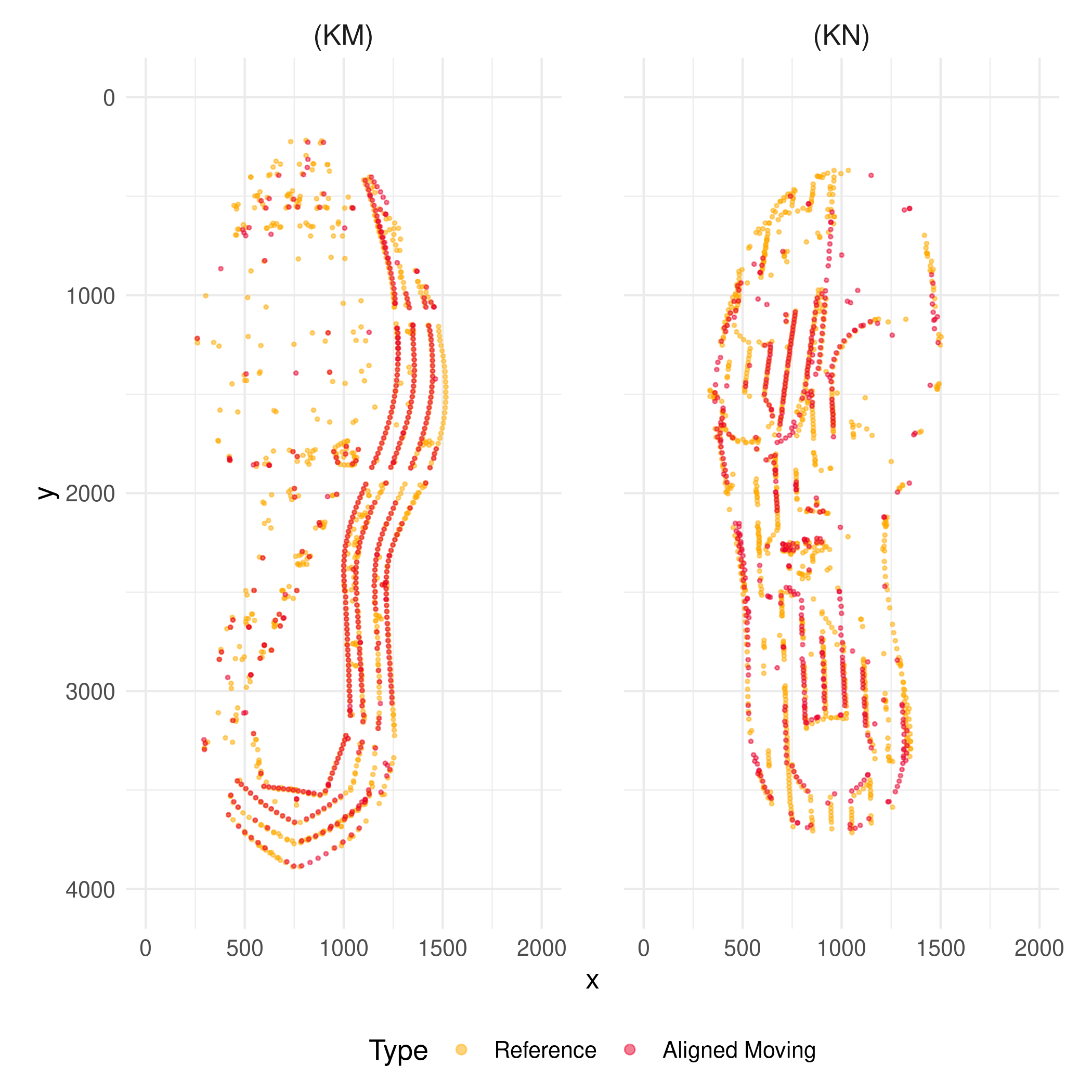Figure 1. The left and right panels present the reference SURF points with the moving SURF points aligned to it based on a known matching pair (KM), and a known nonmatching pair (KN), respectively where a thousand of the strongest SURF points from a reference image, and five hundreds of the strongest SURF points from a moving image are shown.

The first stage is to extract five hundreds of points of SURF from each of two images of shoe outsoles compared, and to align the two sets of points by ICP method. As its name indicates, ICP method aligns two sets of SURF points by minimizing sum of the closest distance between the two sets of points. It consequently overlays the SURFs from two outsole images that are similar like human examiners try to overlay the outlines of shoes prior to comparison by lining up potential stationary points that are commonly located in both sets of points. The alignment of SURF points from a known matching pair (KM), and a known nonmatching pair (KN) is presented in Figure 1. Such alignment based on SURF can be applied to the original images, and the results are illustrated in Figures 2, and 3. Note particularly that the outline of both images from (KN), and their common pattern including logos are aligned as intended although the images from two different shoes are not supposed to be perfectly overlapped due to wear-and-tear as well as subtle difference in the design resulting from the production process.

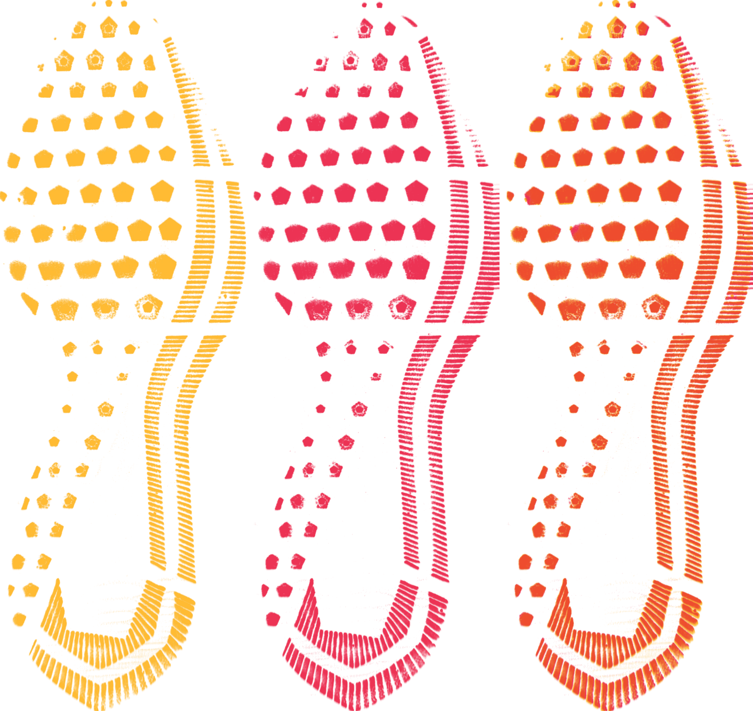Figure 2. The most left image colored in yellow is a reference, and the middle colored in red is a moving image aligned to the reference by ICP method based on SURF for the case of (KM). The most right panel shows the reference overlaid with the aligned moving image.

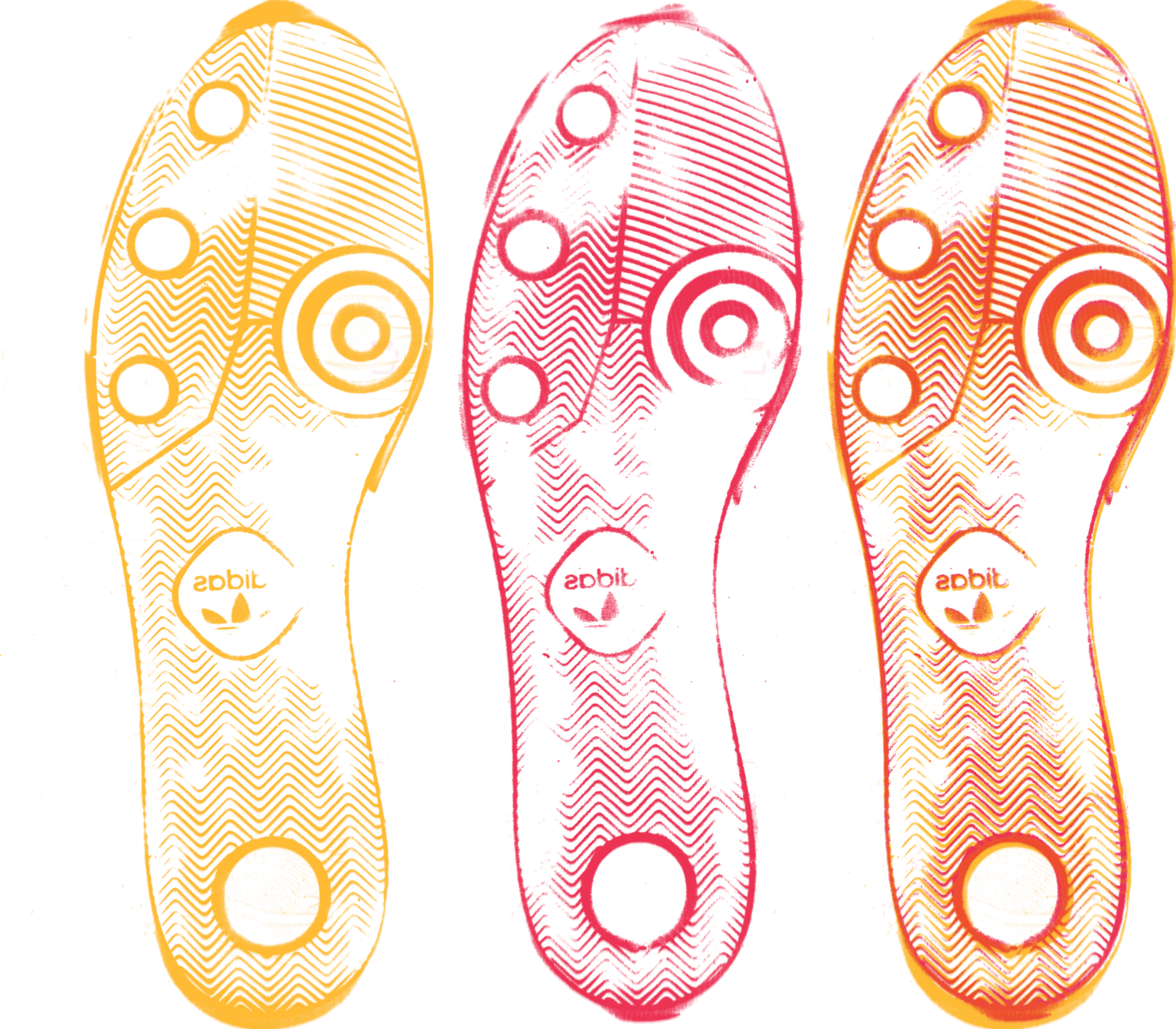Figure 3. The most left image colored in yellow is a reference, and the middle colored in red is a moving image aligned to the reference by ICP method based on SURF for the case of (KN). The most right panel shows the reference overlaid with the aligned moving image.

Next, the features from the aligned SURFs and images are computed where a double number of reference SURF points are used. The closest distances from each of the aligned moving SURF points to the reference SURF points, and then their first quantile, and average are used as features. In addition to that, the average number of neighboring reference SURF points around each of the aligned moving SURF points within a set of small distances is calculated, and their mean across the distances is taken as a feature. Likewise, the average number of the aligned moving SURF points that have no neighborihg reference SURF points within the set of small distances is obtained, and their mean across the distances is used as a feature. Lastly, the phase only correlation between the aligned images is considered to be a feature, which is a key feature to distinguish matching and nonmatching pairs by this algorithm.

The proposed algorithm was applied to two datasets denoted by Dataset1, and Dataset2 and its performance to distinguish matching and nonmatching pairs was compared with that of the algorithm based on maximum cliques and randomforest denoted by MC developed by Park and Carriquiry (2020) that had demonstrated high accuracy rate. Both datasets consist of about 420 of matching and close nonmatching pairs made by Nike shoes, and Adidas shoes in various sizes whose designs are the same as shown in Figure 2 and 3 where a matching pair and a close nonmatching pair indicate two outsole images from the same shoe, and from two different shoes whose class characteristics including design, size, and side are identical, respectively. The two images in each matching pair of Dataset1 are just replicated scans of the same shoe, meaning that the second scan was obtained immediately after the first one was made. On the other hand, the one image of each matching pair of Dataset2 was created several months after the other scan was created so that the degree of wear-and-tear of the same shoe is different between the two scanned images. Hence, Dataset2 would be more challenging than Dataset1 for the algorithms to identify the source of shoe outsole images in a sense that the two images from the same shoe are less similar in Dataset2. Each dataest was split into a training set independent of a test set by brand, and the predictive performance of the randomforest based on a training set (Nike) was evaluated on the test set (Adidas). Figure 4 displays the performance of the proposed algorithm and MC algorithm, illustrating that the MC algorithm is slightly better than or comparable to the proposed algorithm on Dataset1, but the proposed method is superior with the higher ROC curve on Dataset2. Note also that when the features from both algorithms are used together, the ROC curves are improved on Dataset2.

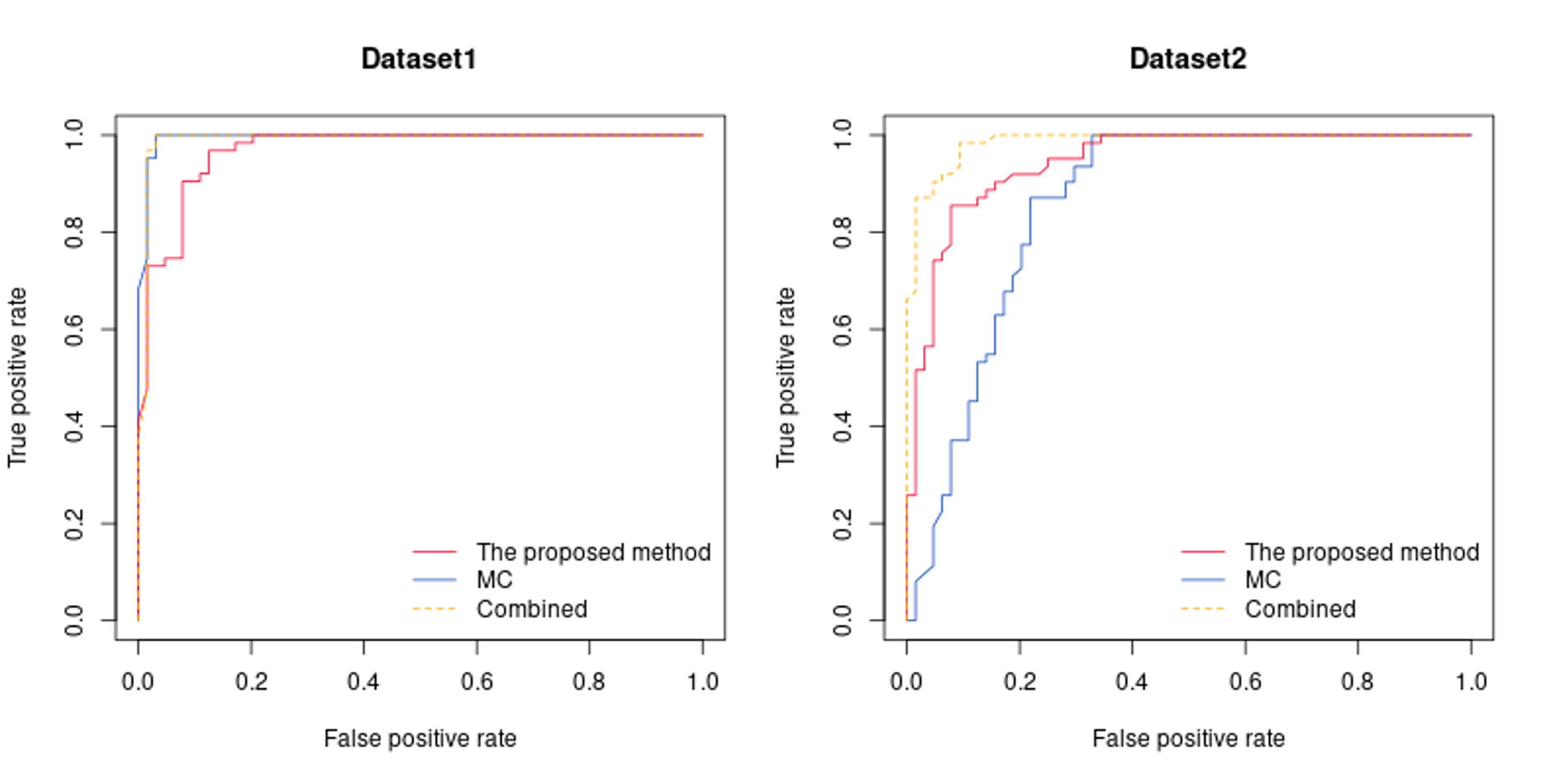Figure 4. ROC curves on Dataset1 and 2 by the proposed method, the algorithm based on MC, and the combination of both are shown. The area under curve (AUC) of each method is 0.969, 0.995, 0.991 on Dataset1, and 0.944, 0.855, 0.986 on Dataset2.

7.9.0.0.1 Hana’s update on 6/16/2022

Figure1. My goal is to align first two images so that the most right images is obtained. Currently, the third image resulted from manual alignment.

Figure2. My approach based on SURF and ICP algorithm provided the following results, which needs improvement.

7.10 Shoe Comparisons through Time

7.10.0.1 NIKE

Definitions: Matched Shoes: When the scans of the same shoes from different time periods are compared

Non-matched shoes: When scans of different shoes from different time periods are compared.

Time Comparison: The visits that are being compared; for example: Visit one compared to visit two. 6 time comparisons in total.

Image Type: The process of how the image was taken. Either the shoe is “stomped” onto the scanner, or the shoe is “rolled” onto the scanner.

Actual Comparisons:By keeping time comparisons and image types separate, we create in total 12 separate groups.

Setup: 1. Create a data frame of matched shoes by creating a data set for each combination of time comparison and image type and then joining all of them together.Used function “matching” to create the data sets.

2. To create the data frame for non-matches I used the number of observations for each combination of time comparison and image type in matched data as n for each corresponding group on non-matched data. Used a stratified random sample design to get the non-matched comparisons using shoe size as the discriminating variable. Allocation of n was proportional.

Average of Variables by Category Image Type 1 Category | Clique Size| Rotation Angle|M-E-D |Overlap| ———|————|—————|——-|——-| match |17.03 | 2.94 |0.83 | 0.52 | non-match| 11.08 | 4.71 |1.29 | 0.23 |

Average of Variables by Category Image Type 2 Category–| Clique Size| Rotation Angle| M-E-D| Overlap| ———-|————|—————|——|——–| match |17.45 |2.85 | 0.82| 0.498 | non-match | 11.19 | 4.2 | 1.32 | 0.21 |

P-value of Anova Tests Comparing Category Variable | Image Type 1| Image Type 2| —————–|————-|————-| Clique Size |≈0 |≈0 | —————–|————-|————-| Reference Overlap|≈0 |≈0 | —————–|————-|————-| M-E_D |≈0 |≈0 | —————–|————-|————-| Rotation Angle |≈0 |≈0 |

Random Forest for Image Type One

Full data set contained all time comparisons for image type one. Data was split into 80%(1073 observations) training, 20% testing(269 observations).

Confusion Matrix; Testing Set | Predicted | —————————–| Observed | Match| Non-match| ———|——–|———-| Match | 124 | 15 | ———|——–|———-|
Non-Match| 8 | 122 |

RF model has an accuracy of 91.4%

RF Variable Importance

Variable	Mean Decrease Gini
Clique Size	96.52512
Rotation Angle	18.91749
Overlap %	266.33528
Median Euclidean Distance	52.46551

Random Forest Model for Image Type 2

Full data set used contained all time comparisons for image type two. Data was split into 80%(1043 observations) training, 20% testing(261 observations).

     |   Predicted   |

———|—————| Observed |match|non-match| ———|—–|———| match | 127 | 7 | ———|—–|———| non-match| 5 | 122 |

The RF model has an classification accuracy of 95.4%

####Round Robin Updates

February 8th,2020 Matias Ibarburu I finished creating data sets for Nike shoes. I created 6 dataframes, one for each shoe image and visit comparison. These are better than my prior Nike data frames because they only compare shoes of the same size. These data frames also have the advantage that each shoe size has the same proportion in each data frame, and is the same proportion that each size appears in the longitudinal study. The matched comparisons and the non-matched comparisons have equal representation in each dataset.

February 15th 2020, Matias Ibarburu I am in the process of analyzing and writing up the datasets I have created for Nike.

7.11 Methods to Address Dependence in Score-based Likelihood Ratios (SLRs)

The score-based likelihood ratio (SLR) and the likelihood ratio (LR) are two ways of quantifying the strength of evidence and have been used in many areas of forensics, including footwear analysis. In forensics, the SLR is distinguished from the LR in that the SLR uses ``scores” that are computed from pairs, instead of the features used by the LR. (The features used in the LR are from individuals.) For example, the LR may use the heights of individuals, while the SLR uses the difference in heights between pairs of individuals. Often, the SLR also only uses one score instead of the multiple features used in the LR, providing lower dimensionality when compared with the LR.

Given scores \(s_1,\dots, s_k\) where each \(s_i\) is computed from a pair of shoeprints \(A\) and \(B\), the SLR is defined as \[\begin{equation*} \textrm{SLR} = \frac{f(s_1,\dots, s_k| A,B \textrm{ are from the same shoe})}{f(s_1,\dots, s_k| A,B \textrm{ are from different shoes})}, \end{equation*}\] where \(f(s_1,\dots, s_k| A,B \textrm{ are from the same shoe})\) and\ \(f(s_1,\dots, s_k| A,B \textrm{ are from different shoes})\) are densities for the scores \(s_1,\dots, s_k\) under two different hypotheses.

In order to estimate the SLR, each of these densities must be estimated using a background population. Scores are computed from pairs from the dataset and then the density of those scores is estimated. In general, the scores do not follow a known parametric form, especially when \(k\geq 2\). Kernel density estimation (KDE) is a common nonparametric method of density estimation. However, as with most density estimation methods, the data are assumed to be independent. Scores computed from pairs are not independent when those individuals repeat in the pairs. Although we may naively take a small independent set of pairs to compute independent scores, this drastically reduces the size of our dataset. Our research centers on exploring how the dependence affects the accuracy of the SLR and on developing methods that address the dependence without discarding such a large part of the dataset.

This research focuses on footwear evidence, though the methods of dealing with dependence are more widely applicable. We use the CSAFE footwear dataset. Park and Carriquiry (2020) proposed a method based on the idea of a maximal clique to find the best alignment for a pair of shoeprint images. Once two images are aligned, variables can be measured that may help quantify the closeness between the aligned images. Three variables are considered: maximal clique size, percent of overlapping features in the two images, and median Euclidean distance between overlapping features.

Two ``default” methods:

1. Ignoring dependence

2. Naive independent set

Three proposed methods:

1. Average each of the three variables over pairs of shoes

2. Independent set for bandwidth selection

3. Computing KDE for multiple independent sets and averaging the estimated densities

Recently:

• Obtained results for right/left dependence

• Wrote more: mostly expanded methods and results section

• Realized that KM data is missing a lot of right shoes for some reason