Integrating handwriter into a workflow

Interested in how to integrate handwriter into your own project?

This page will give you a little more information on integration, as well as an example of how we used it

Inputs & Outputs

As an input, handwriter take a .png image of handwriting. To input a .png image into handwriter, please follow the steps described in the methods section. As a result, handwriter outputs the information and measurements for each graph as a list of lists. You will want to keep this in mind as you integrate handwriter into your own workflow

How we use it

The handwriter package is one of the tools in the larger system to automate the examination of handwritten samples. Depending on the type of question on which the examiner is interested, the steps in the workflow may vary. In all cases however, decomposing handwritten samples into graphical structures that are amenable for quantitative analyses using handwriter is a required step. Roughly, we can think of three major components in the workflow:

1. Data Collection
   • Collect handwriting samples
   • Scan, load, and crop images via batch processing
2. Computational Tools
• Binarize: Turn image to black and white
• Skeltonize: Reduce writing to 1 pixel wide
• Break into graphs: Decompose into managable pieces
• Measure: Extract various measurements of these graphs
3. Statistical analysis
• Clustering: Separate graphs based on shape
• Model: Fit a statistical model to the data
• Quantify: Compute the probability of writership of a questioned document.

Step 1: Data Collection

We are conducting a large data collection study to gather handwriting samples from a variety of participants across the world (most in the Midwest). Each participant provides replicate handwriting samples during three sessions separated by about a month. They also provide other information (e.g., time of day in which writing was done) by filling out a short survey.

Once recieved, we scan all surveys and writing samples. Scans are loaded, cropped, and saved using a Shiny app. The app also facilitates survey data entry, saving that participant data to lines in an excel spreadsheet.

A public database of handwriting samples we have collected can be found at forensicstats.org/handwritingdatabase.

A data article regarding these samples was accepted at Data in Brief
Crawford, A., Ray, A., & Carriquiry, A. (2020). A database of handwriting samples for applications in forensic statistics. Data in brief, 28, 105059.

Step 2: Computational Tools

Information on computational tools can be found in the methods section.

Step 3: Statistical Analysis

Clustering

Rather than impose rigid grouping rules (the previously used ‘’adjacency grouping’’) we consider a more robust, dynamic K − means type clustering method that is focused on major graph structural components.

For a clustering algorithm we need two things:

1. A distance measure - For us, a way to measure the discrepency between graphs.
2. A measure of center - A graph-like structure that is the exemplar representation of a group of graphs.

Graph Distance Measurement

We begin by defining edge to edge distances. Edge to edge distances are subsequently combined for an overall graph to graph distance.

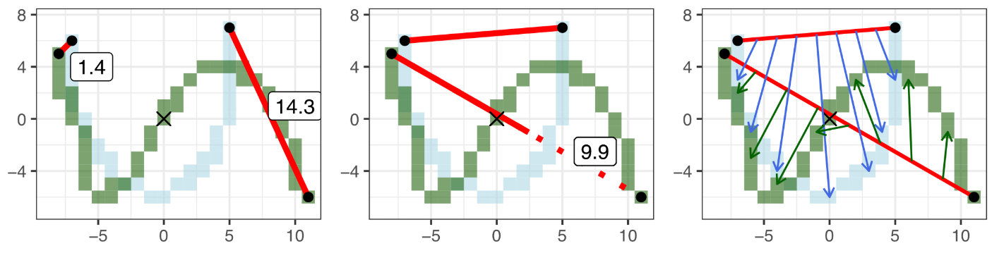
Consider the following single edge graphs e1 and e2. Make 3 edits to e1 to match e2. Then combine the magnitude of each edit.

Measure 1 (Left) - Shift: Anchor to the nearest endpoint by shifting. In our example, the shift value is 1.4.

Measure 2 (Center) - Stretch: Make the end points the same distance apart. Stretch value of 9.9.

Measure 3 (Right and Bottom) - Shape: Bend and twist the edge using 7 shape points. Shape points are 'matched' and the distance between them is averaged to obtain the shape value. Shape value of 8.4 after averaging

Shape measurements averaged

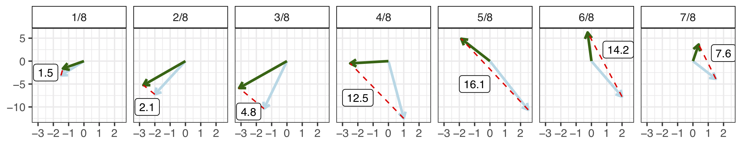
So, our edge to edge distance: D(e1, e2) = 1.4 + 9.9 + 8.4 = 19.7

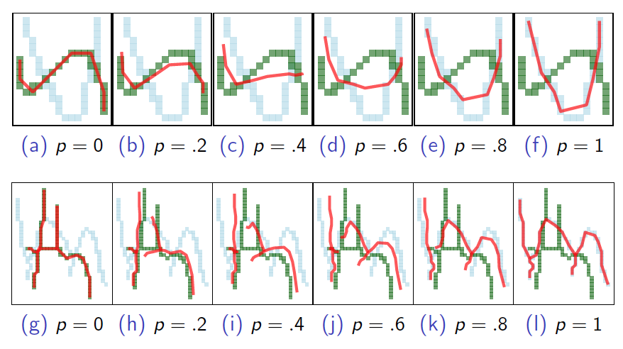
Measure of graph Centers

For this measurement, we take the weighted average of endpoints, 7 shape points, and edge length

K-means clustering algorithm for graphs

We implement a standard K-means. We begin with a fixed K and set of exemplars. Iterate between the following steps until cluster assignments don't change:

1. Assign each graph to the cluster anchored by the nearest exemplar using the distance measure defined earlier

2. Calculate the new cluster means as described above and find the exemplar graph that is nearest the new mean.

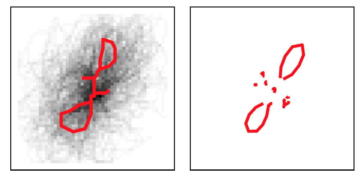
An example cluster when K = 40 is shown below. Examplar is shown on the left in red, with other cluster members shown in black in the background. On the right is the cluster mean.

During clustering, outliers are considered graphs that are a certain distance from the exemplar. The algorithm sets a ceiling on the allowable number of outliers.

Statistical Modeling

The modeling approach depends on the forensic question of interest. If the goal is to identify the most likely author of a questioned sample from among a closed set of potential authors, then the approach that is described in Crawford et al. (2020) and in Crawford et al. (2022) is appropriate. If, however, the problem involves a one-to-many comparison, as in the case of an open set of potential writers, then the methods described in Johnson and Ommen (2022) can be applied. The code to implement all of those statistical modeling approaches can be requested by contacting the manuscript authors. We will eventually include all computational tools as part of the open-source package, once extensive testing and documentation of the programs has been completed.