Advanced ggplot2

class: center, middle, inverse, title-slide

# Advanced <code>ggplot2</code>
### Haley Jeppson and Sam Tyner

---

class: inverse
# Visual Appearance

---
class: primary
# Built-In Themes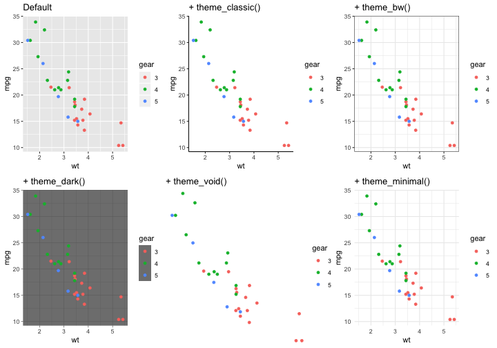

![](06-r-advanced-ggplot2_files/figure-html/unnamed-chunk-2-1.png)

---
class: primary
# Other Themes

`ggthemes`: a `ggplot2` extension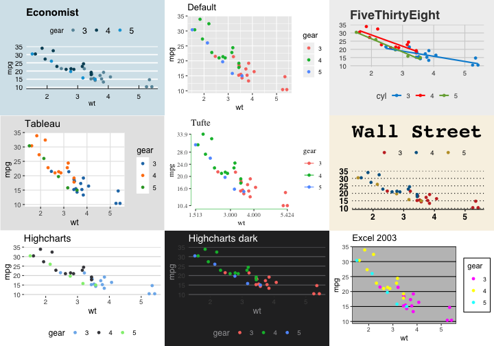

![](06-r-advanced-ggplot2_files/figure-html/unnamed-chunk-3-1.png)

---
class: primary
# Setting Themes

You can globally set a theme with the `theme_set()` function:

```r
theme_set(theme_bw())

ggplot(mtcars, aes(x = wt, y = mpg, colour = gear)) + geom_point()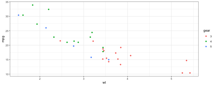
```

![](06-r-advanced-ggplot2_files/figure-html/unnamed-chunk-4-1.png)

---
class: primary
# Elements in a theme

The function `theme()` is used to control non-data parts of the graph including:

- **Line elements**: axis lines, minor and major grid lines, plot panel border, axis ticks background color, etc.  
- **Text elements**: plot title, axis titles, legend title and text, axis tick mark labels, etc.  
- **Rectangle elements**: plot background, panel background, legend background, etc.

.small[
There is a specific function to modify each of these three elements :

- `element_line()` to modify the line elements of the theme
- `element_text()` to modify the text elements
- `element_rect()` to change the appearance of the rectangle elements
- `element_blank()` to draw nothing and assign no space

**Note**: `rel()` is used to specify sizes relative to the parent, `margins()` is used to specify the margins of elements.]

---
class: primary
# Modifying a plot

```r
p1 <- ggplot(mpg) + 
 geom_bar(aes(x = class, colour = manufacturer, fill = manufacturer) )

p2 <- p1 + theme_classic() + theme(
 ## modify plot background
 plot.background = element_rect(fill = "lightskyblue1",colour = "pink",size = 0.5, linetype = "longdash")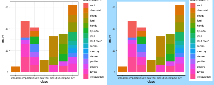
 )
```

![](06-r-advanced-ggplot2_files/figure-html/unnamed-chunk-6-1.png)

---
class: primary
# Plot Legends

```r
p3 <- p2 + theme(
 ### move and modify legend 
 legend.title = element_blank(),
 legend.position = "top", 
 legend.key = element_rect(fill = "lightskyblue1", color = "lightskyblue1"),
 legend.background = element_rect( fill = "lightskyblue1",color = "pink", size = 0.5,linetype = "longdash")
 )
```

![](06-r-advanced-ggplot2_files/figure-html/unnamed-chunk-8-1.png)

---
class: primary
# Modifying Axes

```r
p4 <- p3 + theme(
 ### remove axis ticks
 axis.ticks=element_blank(),
 ### modify axis lines
 axis.line.y = element_line(colour = "pink", size = 1, linetype = "dashed"),
 axis.line.x = element_line(colour = "pink", size = 1.2, linetype = "dashed"))
```

![](06-r-advanced-ggplot2_files/figure-html/unnamed-chunk-10-1.png)

---
class: primary
# Plot Labels

Can be modified in several ways:
- `labs()`, `xlab()`, `ylab()`, `ggtitle()`
- You can also set axis and legend labels in the individual scales (using the first argument, the name)
.

```r
p5 <- p4 + labs(x = "Class of car", 
 y = "",
 title = "Cars by class and manufacturer",
 subtitle = "With a custom theme!!")
```

![](06-r-advanced-ggplot2_files/figure-html/unnamed-chunk-12-1.png)

---
class: primary
# Zooming

```r
p <- ggplot(mtcars, aes(x = wt, y = mpg, colour = gear)) + geom_point() 
p_zoom_in <- p + xlim(2, 4) + ylim(10, 25)
p_zoom_out <- p + xlim(0,7) + ylim(0, 45)
```

![](06-r-advanced-ggplot2_files/figure-html/unnamed-chunk-14-1.png)

---
class: inverse
# Interactive graphics

---
class: primary
# Plotly

```r
p <- ggplot(mtcars, aes(x = wt, y = mpg, colour = gear)) + geom_point() + scale_color_locuszoom()

library(plotly)
ggplotly(p)
```

<div id="htmlwidget-00ad75613932fba8642a" style="width:720px;height:252px;" class="plotly html-widget"></div>
<script type="application/json" data-for="htmlwidget-00ad75613932fba8642a">{"x":{"data":[{"x":[3.215,3.44,3.46,3.57,4.07,3.73,3.78,5.25,5.424,5.345,2.465,3.52,3.435,3.84,3.845],"y":[21.4,18.7,18.1,14.3,16.4,17.3,15.2,10.4,10.4,14.7,21.5,15.5,15.2,13.3,19.2],"text":["wt: 3.215 mpg: 21.4 gear: 3","wt: 3.440 mpg: 18.7 gear: 3","wt: 3.460 mpg: 18.1 gear: 3","wt: 3.570 mpg: 14.3 gear: 3","wt: 4.070 mpg: 16.4 gear: 3","wt: 3.730 mpg: 17.3 gear: 3","wt: 3.780 mpg: 15.2 gear: 3","wt: 5.250 mpg: 10.4 gear: 3","wt: 5.424 mpg: 10.4 gear: 3","wt: 5.345 mpg: 14.7 gear: 3","wt: 2.465 mpg: 21.5 gear: 3","wt: 3.520 mpg: 15.5 gear: 3","wt: 3.435 mpg: 15.2 gear: 3","wt: 3.840 mpg: 13.3 gear: 3","wt: 3.845 mpg: 19.2 gear: 3"],"type":"scatter","mode":"markers","marker":{"autocolorscale":false,"color":"rgba(212,63,58,1)","opacity":1,"size":5.66929133858268,"symbol":"circle","line":{"width":1.88976377952756,"color":"rgba(212,63,58,1)"}},"hoveron":"points","name":"3","legendgroup":"3","showlegend":true,"xaxis":"x","yaxis":"y","hoverinfo":"text","frame":null},{"x":[2.62,2.875,2.32,3.19,3.15,3.44,3.44,2.2,1.615,1.835,1.935,2.78],"y":[21,21,22.8,24.4,22.8,19.2,17.8,32.4,30.4,33.9,27.3,21.4],"text":["wt: 2.620 mpg: 21.0 gear: 4","wt: 2.875 mpg: 21.0 gear: 4","wt: 2.320 mpg: 22.8 gear: 4","wt: 3.190 mpg: 24.4 gear: 4","wt: 3.150 mpg: 22.8 gear: 4","wt: 3.440 mpg: 19.2 gear: 4","wt: 3.440 mpg: 17.8 gear: 4","wt: 2.200 mpg: 32.4 gear: 4","wt: 1.615 mpg: 30.4 gear: 4","wt: 1.835 mpg: 33.9 gear: 4","wt: 1.935 mpg: 27.3 gear: 4","wt: 2.780 mpg: 21.4 gear: 4"],"type":"scatter","mode":"markers","marker":{"autocolorscale":false,"color":"rgba(238,162,54,1)","opacity":1,"size":5.66929133858268,"symbol":"circle","line":{"width":1.88976377952756,"color":"rgba(238,162,54,1)"}},"hoveron":"points","name":"4","legendgroup":"4","showlegend":true,"xaxis":"x","yaxis":"y","hoverinfo":"text","frame":null},{"x":[2.14,1.513,3.17,2.77,3.57],"y":[26,30.4,15.8,19.7,15],"text":["wt: 2.140 mpg: 26.0 gear: 5","wt: 1.513 mpg: 30.4 gear: 5","wt: 3.170 mpg: 15.8 gear: 5","wt: 2.770 mpg: 19.7 gear: 5","wt: 3.570 mpg: 15.0 gear: 5"],"type":"scatter","mode":"markers","marker":{"autocolorscale":false,"color":"rgba(92,184,92,1)","opacity":1,"size":5.66929133858268,"symbol":"circle","line":{"width":1.88976377952756,"color":"rgba(92,184,92,1)"}},"hoveron":"points","name":"5","legendgroup":"5","showlegend":true,"xaxis":"x","yaxis":"y","hoverinfo":"text","frame":null}],"layout":{"margin":{"t":36.8741030658839,"r":7.30593607305936,"b":50.8284409654273,"l":37.2602739726027},"plot_bgcolor":"rgba(255,255,255,1)","paper_bgcolor":"rgba(255,255,255,1)","font":{"color":"rgba(0,0,0,1)","family":"","size":14.6118721461187},"xaxis":{"domain":[0,1],"automargin":true,"type":"linear","autorange":false,"range":[1.31745,5.61955],"tickmode":"array","ticktext":["2","3","4","5"],"tickvals":[2,3,4,5],"categoryorder":"array","categoryarray":["2","3","4","5"],"nticks":null,"ticks":"outside","tickcolor":"rgba(51,51,51,1)","ticklen":3.65296803652968,"tickwidth":0.66417600664176,"showticklabels":true,"tickfont":{"color":"rgba(77,77,77,1)","family":"","size":11.689497716895},"tickangle":-0,"showline":false,"linecolor":null,"linewidth":0,"showgrid":true,"gridcolor":"rgba(235,235,235,1)","gridwidth":0.66417600664176,"zeroline":false,"anchor":"y","title":"wt","titlefont":{"color":"rgba(0,0,0,1)","family":"","size":14.6118721461187},"hoverformat":".2f"},"yaxis":{"domain":[0,1],"automargin":true,"type":"linear","autorange":false,"range":[9.225,35.075],"tickmode":"array","ticktext":["10","15","20","25","30","35"],"tickvals":[10,15,20,25,30,35],"categoryorder":"array","categoryarray":["10","15","20","25","30","35"],"nticks":null,"ticks":"outside","tickcolor":"rgba(51,51,51,1)","ticklen":3.65296803652968,"tickwidth":0.66417600664176,"showticklabels":true,"tickfont":{"color":"rgba(77,77,77,1)","family":"","size":11.689497716895},"tickangle":-0,"showline":false,"linecolor":null,"linewidth":0,"showgrid":true,"gridcolor":"rgba(235,235,235,1)","gridwidth":0.66417600664176,"zeroline":false,"anchor":"x","title":"mpg","titlefont":{"color":"rgba(0,0,0,1)","family":"","size":14.6118721461187},"hoverformat":".2f"},"shapes":[{"type":"rect","fillcolor":"transparent","line":{"color":"rgba(51,51,51,1)","width":0.66417600664176,"linetype":"solid"},"yref":"paper","xref":"paper","x0":0,"x1":1,"y0":0,"y1":1}],"showlegend":true,"legend":{"bgcolor":"rgba(255,255,255,1)","bordercolor":"transparent","borderwidth":1.88976377952756,"font":{"color":"rgba(0,0,0,1)","family":"","size":11.689497716895},"y":0.876265466816648},"annotations":[{"text":"gear","x":1.02,"y":1,"showarrow":false,"ax":0,"ay":0,"font":{"color":"rgba(0,0,0,1)","family":"","size":14.6118721461187},"xref":"paper","yref":"paper","textangle":-0,"xanchor":"left","yanchor":"bottom","legendTitle":true}],"hovermode":"closest","barmode":"relative"},"config":{"doubleClick":"reset","modeBarButtonsToAdd":[{"name":"Collaborate","icon":{"width":1000,"ascent":500,"descent":-50,"path":"M487 375c7-10 9-23 5-36l-79-259c-3-12-11-23-22-31-11-8-22-12-35-12l-263 0c-15 0-29 5-43 15-13 10-23 23-28 37-5 13-5 25-1 37 0 0 0 3 1 7 1 5 1 8 1 11 0 2 0 4-1 6 0 3-1 5-1 6 1 2 2 4 3 6 1 2 2 4 4 6 2 3 4 5 5 7 5 7 9 16 13 26 4 10 7 19 9 26 0 2 0 5 0 9-1 4-1 6 0 8 0 2 2 5 4 8 3 3 5 5 5 7 4 6 8 15 12 26 4 11 7 19 7 26 1 1 0 4 0 9-1 4-1 7 0 8 1 2 3 5 6 8 4 4 6 6 6 7 4 5 8 13 13 24 4 11 7 20 7 28 1 1 0 4 0 7-1 3-1 6-1 7 0 2 1 4 3 6 1 1 3 4 5 6 2 3 3 5 5 6 1 2 3 5 4 9 2 3 3 7 5 10 1 3 2 6 4 10 2 4 4 7 6 9 2 3 4 5 7 7 3 2 7 3 11 3 3 0 8 0 13-1l0-1c7 2 12 2 14 2l218 0c14 0 25-5 32-16 8-10 10-23 6-37l-79-259c-7-22-13-37-20-43-7-7-19-10-37-10l-248 0c-5 0-9-2-11-5-2-3-2-7 0-12 4-13 18-20 41-20l264 0c5 0 10 2 16 5 5 3 8 6 10 11l85 282c2 5 2 10 2 17 7-3 13-7 17-13z m-304 0c-1-3-1-5 0-7 1-1 3-2 6-2l174 0c2 0 4 1 7 2 2 2 4 4 5 7l6 18c0 3 0 5-1 7-1 1-3 2-6 2l-173 0c-3 0-5-1-8-2-2-2-4-4-4-7z m-24-73c-1-3-1-5 0-7 2-2 3-2 6-2l174 0c2 0 5 0 7 2 3 2 4 4 5 7l6 18c1 2 0 5-1 6-1 2-3 3-5 3l-174 0c-3 0-5-1-7-3-3-1-4-4-5-6z"},"click":"function(gd) { \n // is this being viewed in RStudio?\n if (location.search == '?viewer_pane=1') {\n alert('To learn about plotly for collaboration, visit:\\n https://cpsievert.github.io/plotly_book/plot-ly-for-collaboration.html');\n } else {\n window.open('https://cpsievert.github.io/plotly_book/plot-ly-for-collaboration.html', '_blank');\n }\n }"}],"cloud":false},"source":"A","attrs":{"e16762fe79fa":{"x":{},"y":{},"colour":{},"type":"scatter"}},"cur_data":"e16762fe79fa","visdat":{"e16762fe79fa":["function (y) ","x"]},"highlight":{"on":"plotly_click","persistent":false,"dynamic":false,"selectize":false,"opacityDim":0.2,"selected":{"opacity":1}},"base_url":"https://plot.ly"},"evals":["config.modeBarButtonsToAdd.0.click"],"jsHooks":[]}</script>

---
class: inverse
# Saving graphics

---
class: primary
# Saving your Work

We can save the results of a plot to a file (as an image) using the `ggsave()` function:

```r
p1 <- ggplot(mtcars, aes(x = wt, y = mpg, colour = gear)) + 
 geom_point()

ggsave("mpg_by_wt.pdf", plot = p1)
```

---

## Your Turn

1. Create a scatterplot of y versus x from the `diamonds` data, colored by clarity
2. Use the black and white theme
3. Include an informative title
4. Move the legend to the bottom
5. Save your plot to a pdf file and open it in a pdf viewer.

```r
ggplot(data = diamonds, aes(x = x, y = y))
```

![](06-r-advanced-ggplot2_files/figure-html/unnamed-chunk-17-1.png)