Reading Files

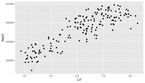
class: center, middle, inverse, title-slide

# Reading Files
### Sam Tyner, Haley Jeppson
### 2018/06/06

---

class: primary
# Data in Excel

- Formats xls and csv - what's the difference?

- File extensions xls and xlsx are proprietary Excel formats, binary files

- csv is an extension for Comma Separated Value files. They are text files - directly readable.

- Example: Glass element analysis data

---
class: primary
# Glass data

Visit [this link](https://raw.githubusercontent.com/CSAFE-ISU/REU-materials-2018/master/slides/rstats/data/GK_clean_results.csv) to get the data.

```r
library(readr)
glass <- read_csv("https://raw.githubusercontent.com/CSAFE-ISU/REU-materials-2018/master/slides/rstats/data/GK_clean_results.csv")
head(glass)
```

```
## # A tibble: 6 x 20
##   Piece   Rep   Li7   Na23  Mg25  Al27   K39  Ca42  Ti49  Mn55  Fe57  Rb85
##   <int> <int> <dbl>  <int> <int> <int> <dbl> <int> <dbl> <dbl> <int> <dbl>
## 1     1     1  2.77 107280 24610  1622  743. 67570  115.  128.   545  1.04
## 2     1     2  2.93 106760 24290  1620  732. 67220  118.  129.   532  1.07
## 3     1     3  2.73 106500 24410  1639  727. 68120  117.  130.   538  1.08
## 4     1     4  2.69 104740 24520  1632  716. 67410  118.  129.   541  1.16
## 5     1     5  2.71 105670 24400  1624  724. 67610  119.  127.   542  1.14
## 6     2     1  2.44 104790 24380  1639  716. 68040  118.  128.   532  1.05
## # ... with 8 more variables: Sr88 <dbl>, Zr90 <dbl>, Ba137 <dbl>,
## #   La139 <dbl>, Ce140 <dbl>, Nd146 <dbl>, Hf178 <dbl>, Pb208 <dbl>
```

---
class: primary
# `read_csv` vs. `read_*`

`read_csv` is just one way to read a file using the `readr` package:

- `read_delim`: the most generic function. Use the `delim` argument to read a file with any type of delimiter 
- `read_tsv`: read tab separated files 
- `read_lines`: read a file into a vector that has one element per line of the file
- `read_file`: read a file into a single character element
- `read_table`: read a file separated by space

---
class: primary
# Now we can make a plot!

```r
library(ggplot2)
ggplot(glass, 
       aes(x = Li7, y = Na23)) + 
  geom_point()
```

![](03-r-files_files/figure-html/unnamed-chunk-2-1.png)

---
class: primary
# Read Excel Data

Download the boxoffice.xlsx file from [this link](https://github.com/CSAFE-ISU/REU-materials-2018/blob/master/slides/rstats/data/boxoffice.xlsx) and put it in your "LearningR" folder.

Read it in and save it as `boxofc`

```r
library(readxl)
 
boxofc <- read_excel("boxoffice.xlsx")

head(boxofc)
```

```
## # A tibble: 6 x 11
##    Rank Rank.Last.Week Movie  Distributor  Gross Change Thtrs. `Per Thtr.`
##   <dbl> <chr>          <chr>  <chr>        <dbl> <chr>   <dbl>       <dbl>
## 1    1. -1             Split  Universal   2.57e7 -0.36   3199.       8020.
## 2    2. new            A Dog… Universal   1.82e7 <NA>    3059.       5957.
## 3    3. -3             Hidde… 20th Centu… 1.40e7 -0.11   3351.       4179.
## 4    4. new            Resid… Sony Pictu… 1.36e7 <NA>    3104.       4382.
## 5    5. -5             La La… Lionsgate   1.22e7 0.45    3136.       3901.
## 6    6. -2             xXx: … Paramount … 8.60e6 -0.56…  3651.       2356.
## # ... with 3 more variables: `Total Gross` <dbl>, Days <dbl>, Date <dttm>
```

---
class: primary
# `foreign` Package

- Other file formats can be read using the functions from package `foreign`

- SPSS: `read.spss`

- SAS: `read.xport`

- Minitab: `read.mtp`

- Systat: `read.systat`

---
class: primary
# Your Turn 3.1

The NHANES (National Health and Nutrition Survey) publishes data in the SAS xport format:

https://wwwn.cdc.gov/Nchs/Nhanes/continuousnhanes/default.aspx?BeginYear=2013

1. Scroll to the bottom, choose one of the datasets (Demographics, Examination, etc.). Download the Data file (XPT)

2. Use `read.xport()` to load the file into R

3. Briefly examine the dataset you've imported (use `head` or `tail`, etc)

---
class: primary
# Other Data Types

What can you think of?

---
class: primary
# Google Sheets

```r
install.packages("googlesheets")
library(googlesheets)
gap <- gs_key("1D5FK6z7aGukdGRAJQoyuPc2QV5zSJ4oN7oslp_u7YEQ")
gs_browse(gap)
africa <- gs_read(gap, "Africa")
americas <- gs_read(gap, "Americas")
```

```
## # A tibble: 6 x 6
##   country continent  year lifeExp       pop gdpPercap
##   <chr>   <chr>     <dbl>   <dbl>     <dbl>     <dbl>
## 1 Algeria Africa    1952.    43.1  9279525.     2449.
## 2 Algeria Africa    1957.    45.7 10270856.     3014.
## 3 Algeria Africa    1962.    48.3 11000948.     2551.
## 4 Algeria Africa    1967.    51.4 12760499.     3247.
## 5 Algeria Africa    1972.    54.5 14760787.     4183.
## 6 Algeria Africa    1977.    58.0 17152804.     4910.
```

---
class: primary
# Text files 
Data is [here](https://raw.githubusercontent.com/CSAFE-ISU/REU-materials-2018/master/slides/rstats/data/poem.txt)

```r
poem <- read_lines("https://raw.githubusercontent.com/CSAFE-ISU/REU-materials-2018/master/slides/rstats/data/poem.txt")
poem
```

```
## [1] "Because I could not stop for Death -"  
## [2] "He kindly stopped for me -"            
## [3] "The Carriage held but just Ourselves -"
## [4] "and Immortality"
```

---
class: primary
# Your Turn 3.2

Read in the rest of the Google Sheets from the Gapminder data set and combine them into one data set with the `bind_rows()` function in the `dplyr` package. Save it as `gapdata`.

---
class: primary
# Plot `gapdata`

```r
library(ggplot2)
ggplot(data = gapdata) + 
  geom_point(aes(x = log(gdpPercap), y = lifeExp, 
                 color = continent, size = pop)) + 
  facet_wrap(~continent)  + 
  theme(legend.position = c(.75,.25))
```

---
class: secondary